Method 1 – Basics of COUNTIF and COUNTIFS Functions
COUNTIF Function
The COUNTIF function operates with a single range and criterion.
⏩ Apply the below formula to develop a number of cells that satisfy a given criterion.
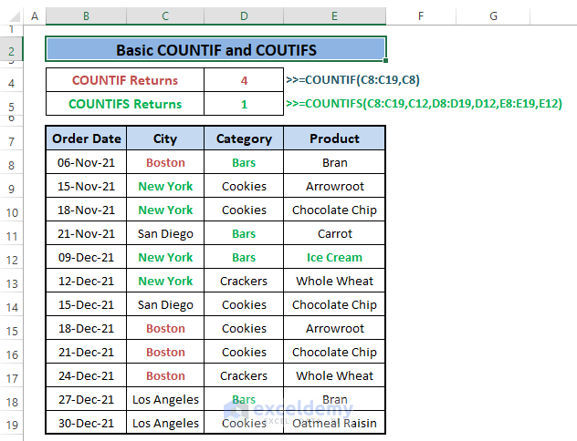
=COUNTIF(C8:C19,C8)In the formula,
C8:C19; is the range.
C8; direct the criterion.
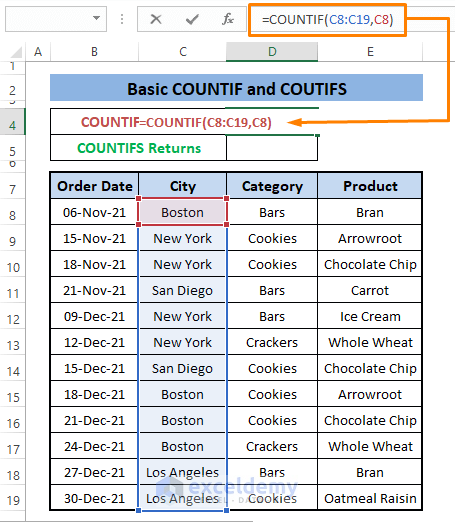
⏩ Press ENTER, the formula counts all the cells containing text “Boston” (i.e., C8).
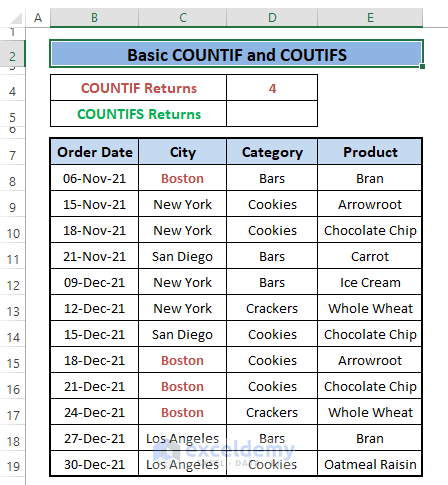
From the dataset, we can see there are 4 matches, and the formula returns 4 maintaining just one criterion i.e. C8.
If you are interested in adding another criterion in the COUNTIF function Excel won’t allow us, you have to use the COUNTIFS function instead.
COUNTIFS Function
Similar to the COUNTIF function the COUNTIFS counts cells, but it allows multiple criteria to be imposed in multiple ranges. Let’s extend the previous criteria we use for COUNTIF. We add another two criteria to fetch the number of cells that match all the requirements imposed.
⏩ Paste the following formula in any cell (i.e., D5).
=COUNTIFS(C8:C19,C9,D8:D19,D8,E8:E19,E12)Inside the formula, we impose three criteria (i.e., C9, D8, & E12) in three different ranges (i.e., C8:C19,D8:D19, & E8:E19).
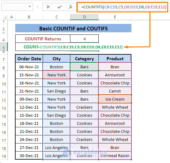
⏩ Hit ENTER, and the number of cells matching all three criteria appears.
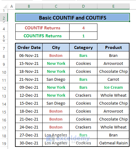
From the dataset, we see only one entry matches all the imposed criteria, as the formula returns. Apply up to 127 criteria; however, for better understanding and representation, apply two or three conditions at a time.
The following image depicts the basic difference between these two functions.
Method 2 – Handling Multiple Criteria with COUNTIF and COUNTIFS
With COUNTIF Function
To insert multiple criteria, we use multiple COUNTIF functions and then assign a criterion in each with a different range,
⏩ Type the following formula in any adjacent cell (i.e., D4).
=COUNTIF(C8:C19,C8)+COUNTIF(D8:D19,D9)+COUNTIF(E8:E19,E10)Use three COUNTIF functions to assign three ranges and criteria.
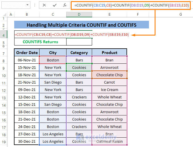
⏩ After Pressing ENTER, the number of matched cells appears similar to the below image.
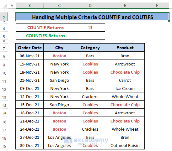
Inspect the dataset, we see the COUNTIF formula adds all the cells that match the criteria to respective ranges, not the number of cells that satisfy all the criteria. It’s the main drawback of the COUNTIF function.
With COUNTIFS Function
If you want to count the number of cells that satisfy the same three criteria using the COUNTIFS function, it returns a different number, and the dataset backs it.
⏩ Write the following formula in any cell (i.e., D5).
=COUNTIFS(C8:C19,C8,D8:D19,D9,E8:E19,E10)The formula declares criteria (i.e., C8,D9,& E10) to match in ranges (i.e., C8:C19,D8:D19, & E8:E19) respectively.
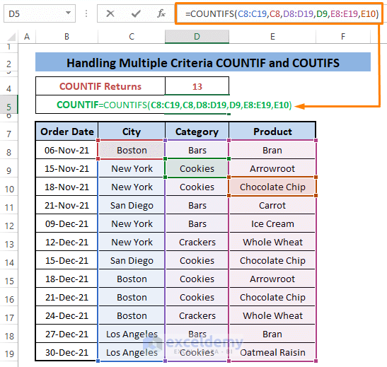
⏩ Hit ENTER, the number of matched cells appears similar to the below picture.
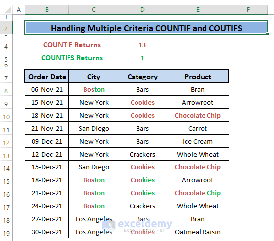
Ensure the result using the dataset that only one entry matches all three criteria.
See the following image as core dissimilarity handling multiple criteria by COUNTIF vs COUNTIFS functions.
Method 3 – Counting Cells with COUNTIF and COUNTIFS
With COUNTIF Function
COUNTIF only counts the non-blank text cells; any imposed condition or certain text can’t be performed.
⏩ Type the following formula in any cell (i.e., D4).
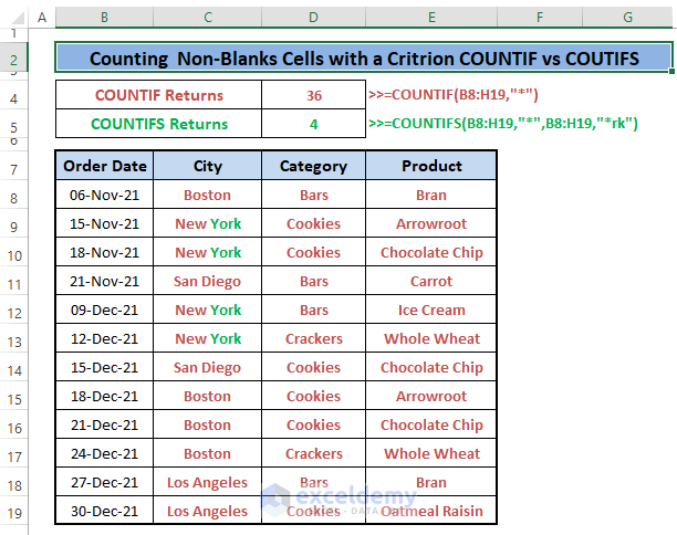
=COUNTIF(B8:E19,"*")“*” enables the formula to count non-blank text cells from the dataset.
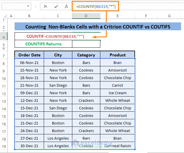
⏩ Hit ENTER, and you will see the number of non-blank text cells shown in the image below.
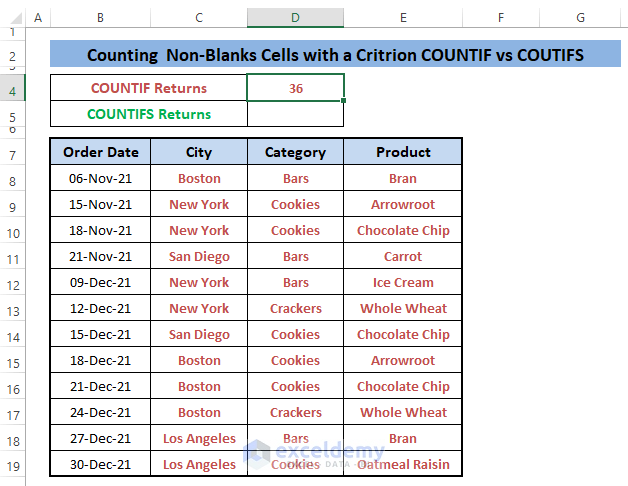
36 text cells are existing in the dataset and the formula returns it.
With COUNTIFS Function
The COUNTIFS function can count the same text non-blank cells as the COUNTIF function does but it offers an option to match the certain text within the text cells.
⏩ Write the below formula in any cell (i.e., D5).
=COUNTIFS(B8:E19,"*",B8:E19,"*rk")“*” enables counting all the text cells within the range and “*rk” matches with text cells with rk at their end.
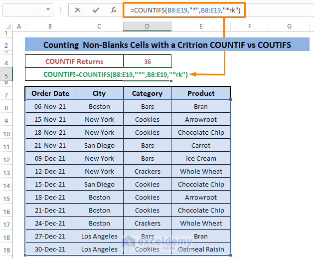
⏩ After Pressing ENTER, you see only 4 entries that have rk at their end as shown in the below picture.
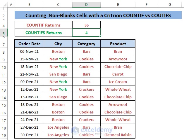
We see commonness in their working process but multi-dimensions in just the COUNTIFS function’s result.
Method 4 – Finding a Match with COUNTIF and COUNTIFS
With COUNTIF Function
The COUNTIF function matches a partial text while we enter the text with wildcards (i.e., *) in the formula. Use other wildcards such as an asterisk (*), question mark (?), and tilde (~).
⏩ Write the following formula in any cell (i.e., D4).
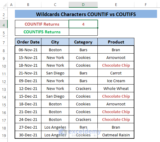
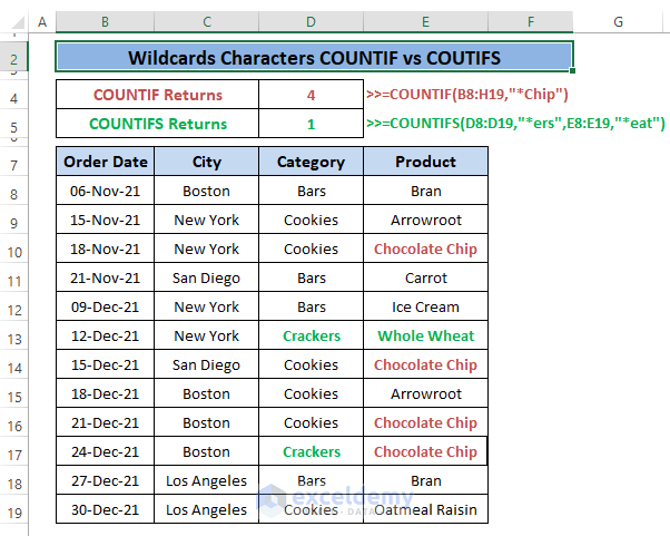
=COUNTIF(B8:E19,"*Chip")The formula matches texts that have Chip at the end. And the “*Chip” works as a criterion.
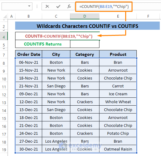
⏩ To bring out the result, Hit ENTER. The matching number of cells that obey the criterion will appear like the picture below.
With COUNTIFS Function
The COUNTIFS matches the text as COUNTIF does additional texts to satisfy the criteria. By combining them we have a match that tends to be very useful searching entries in huge datasets.
⏩ Paste the following formula in any cell (i.e., D5).
=COUNTIFS(D8:D19,"*ers",E8:E19,"*eat")The formula matches both “*ers” and “*eat” in the end within the ranges.
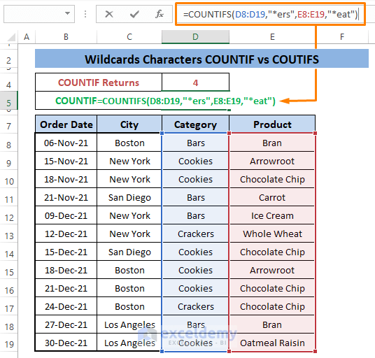
⏩ Press ENTER, and the matched number of the cells appears.
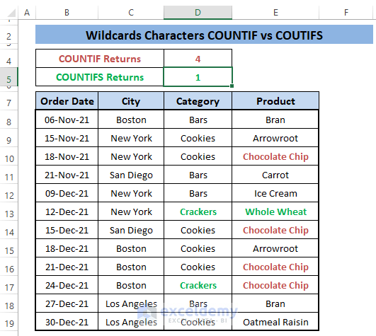
You can tell only one entry matches the imposed criteria.
The picture below offers an overview of what we want to differentiate between the functions. Though it seems to be an example of imposing multiple criteria, we can still use it to find matches from any dataset.
Download Practice Workbook
Further Readings
- How to Use COUNTIF for Non Contiguous Range in Excel
- [Fixed] COUNTIF Function with Wildcard Not Working in Excel
- How to Use Excel COUNTIF Between Time Range (2 Examples)
- COUNTIF Function to Count Cells That Are Not Equal to Zero
- How to Use IF and COUNTIF Functions Together in Excel


