How to Create a General Ledger from a General Data Journal in Excel

What Is a General Journal?

The general journal is an accounting record of a company’s financial transactions. It is the master of all company entities.

What Is a General Ledger?

A general ledger can be used to track specific income and expenses.

Step 1 – Create a General Data Journal

A general data journal consists of date, account, reference, debit, and credit.

• Create the five headings in Excel.

• Select  B4:F4.
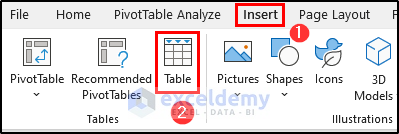
• Go to the Insert tab.
• Select Table in Tables.

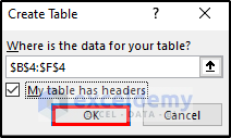
• In the Create Table dialog box, check My table has headers.
• Click OK.

A table is created.

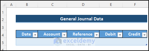
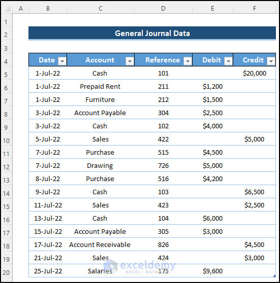
• Add transactions and dates.

This is the general data journal.

To add the Sum of the debit and credit columns:

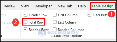
• Select the table and select the Table Design tab.
• Select Total Row in Table Style Options.

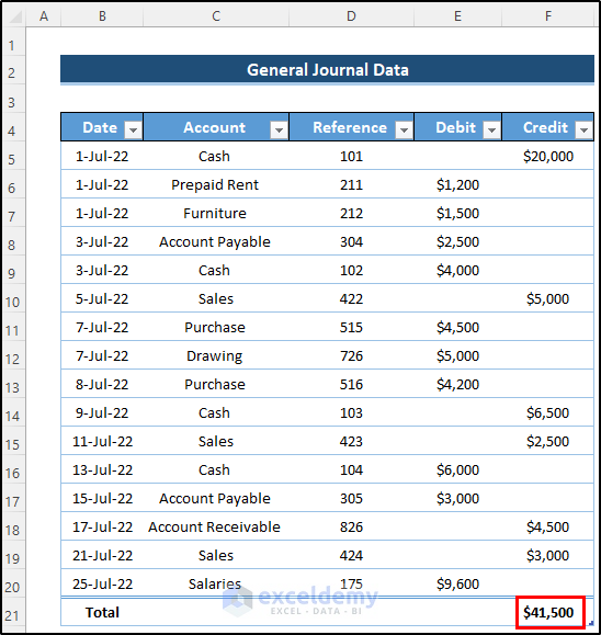
A total will be created in the last column.

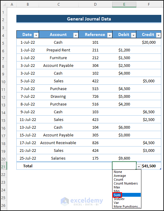
• In the Debit column, you will see a data validation button.
• Click it and select Sum.

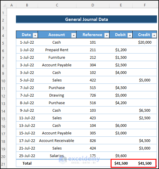
The total in the debit column will be displayed.

Step 2 – Create a Pivot Table

• Go to Insert.
• Select PivotTable in Tables.

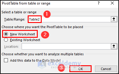
• Select the table or range.
• Choose New Worksheet (in which you will store your PivotTable).
• Click OK.

• The PivotTable Fields dialog box will will be displayed.
• Select all the available options.

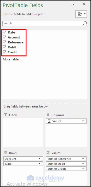
A pivot table will be created from the general data journal.

Step 3 – Modify the Pivot Table

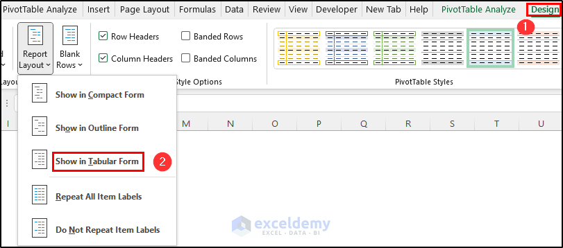
• Select the pivot table and select the Design tab.
• In Layout, choose Report Layout and select Show in Tabular Form.

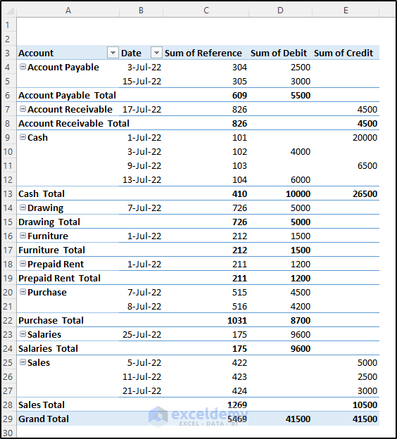
This is the output

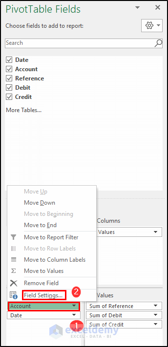
• Go to the PivotTable Fields dialog box.
• Select Account.
• Select Field Settings.

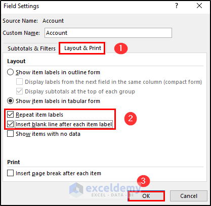
• In the Field Settings dialog box, select Layout & Print.
• Check  Repeats item labels and Insert blank line after each item label.
• Click  OK.

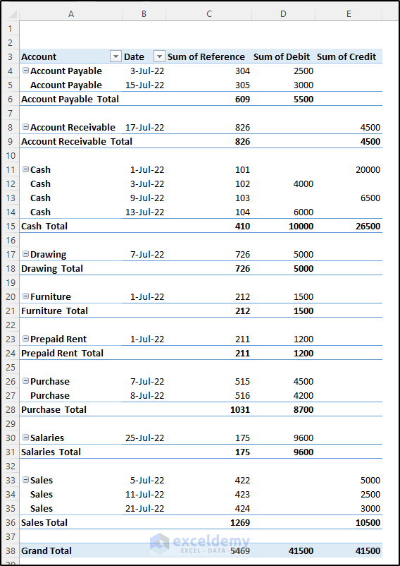
This is the output.

To change the format of the debit and credit columns.

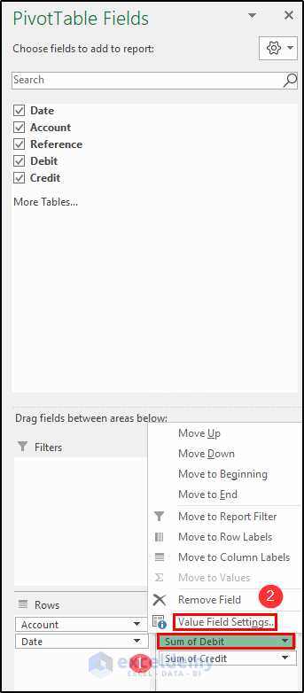
• Go to the PivotTable Fields dialog box and select Sum of Debit.
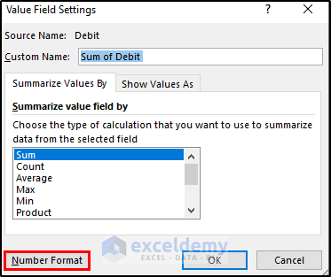
• Choose Value Field Settings.

• In the Value Field Settings dialog box, select Number Format.

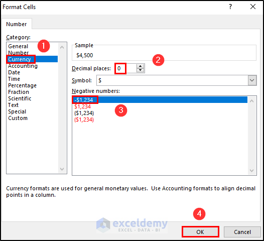
• In the Format Cells dialog box, select Currency in Category.
• Set Decimal places as zero.
• Choose a format for negative numbers.
• Click OK.

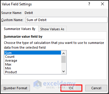
• Click OK in Value Field Settings dialog box.

This is the output

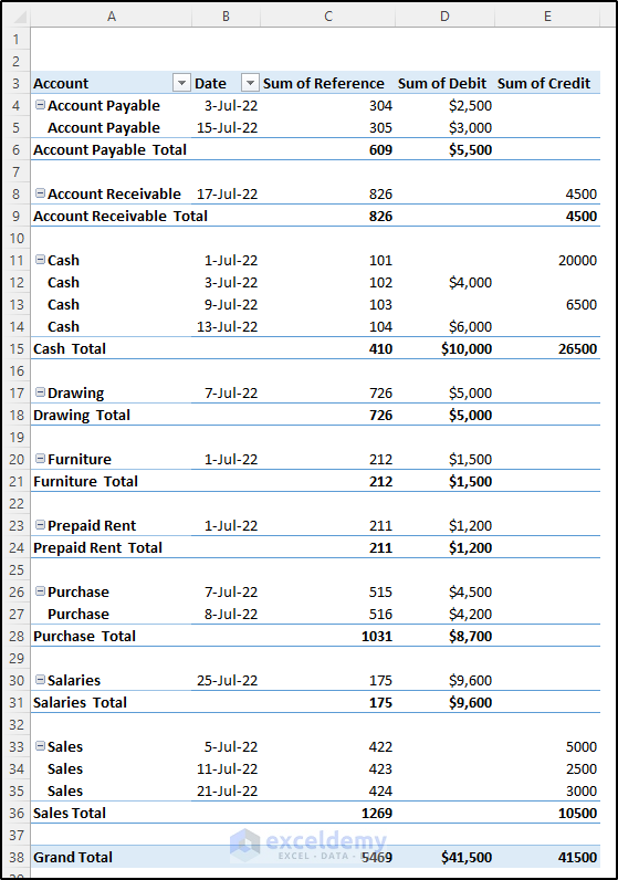
• Follow the same procedure to change the number format in the credit column.

This is the output

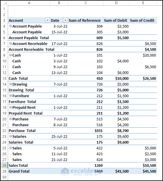
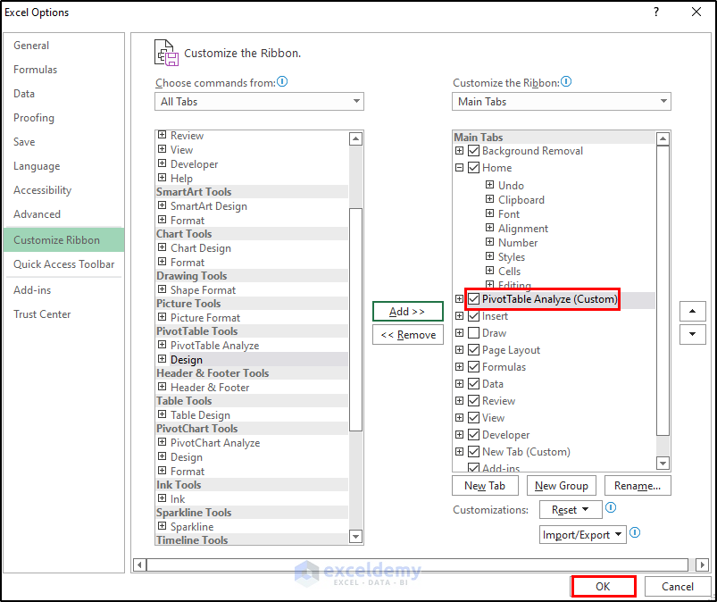
Step 4 – Enable the PivotTable Analyze Tab on the Ribbon

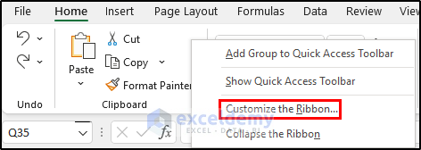
• Right-click the ribbon.
• Select Customize the Ribbon.

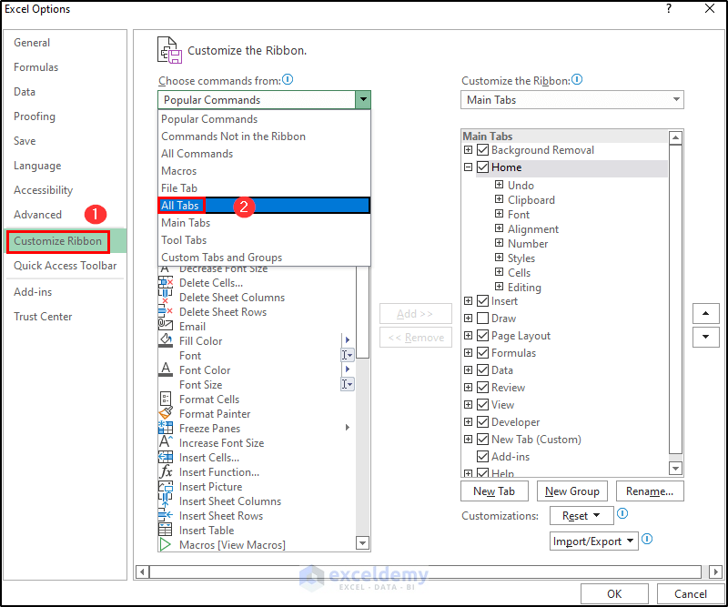
• In the Excel options dialog box, select Customize Ribbon.
• Select All Tabs in Choose commands from.

• Select PivotTable Analyze.
• Click Add.

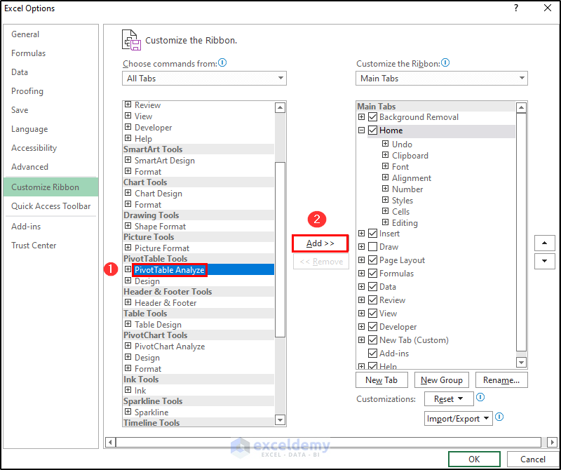
• Click OK.

Step 5 – Create a General Ledger

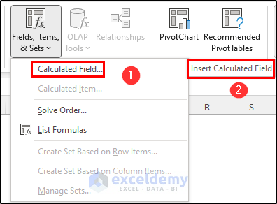
• Select the pivot table.
• Go to the PivotTable Analyze tab.
• Select  Fields, Items & Sets in Calculations.

• Choose Calculated Field and select Insert Calculated Field.

• In the Insert Calculated Field dialog box, set the name and formula.
• Click Add.

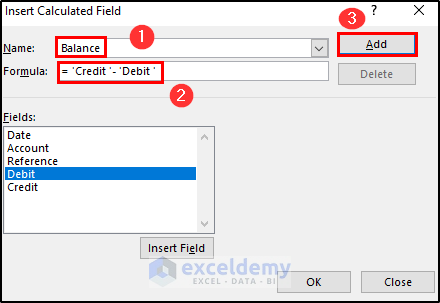
• Click OK.

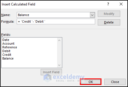
This is the output

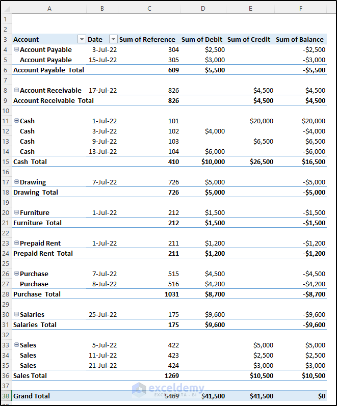
• Go to the PivotTable Analyze tab.
• In Filter, select Insert Slicer.

• Select Account in the Insert Slicers dialog box.
• Click OK.

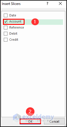
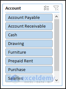
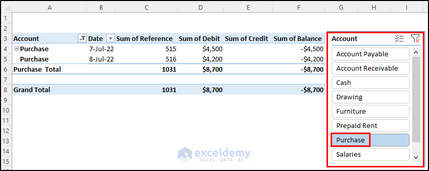
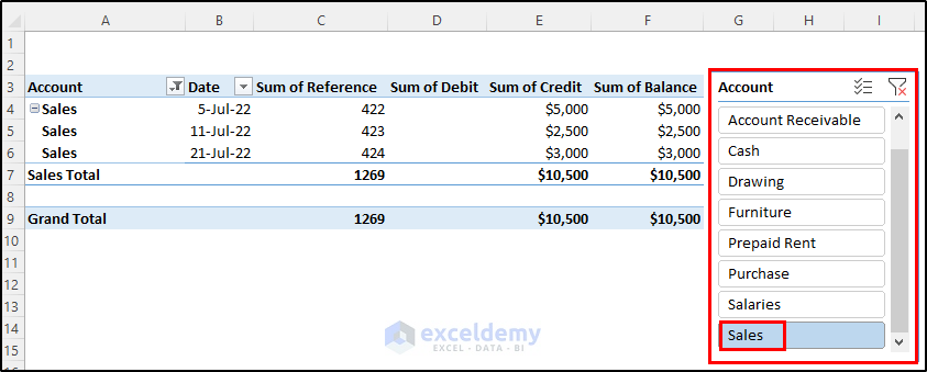
A specific sub-group  will be created.

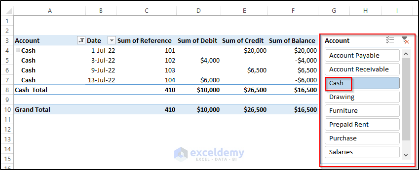
• If you select cash in the slicer, you will see details for cash payments in the general data journal .

• If you choose purchase, you will see purchase transactions.

• Change the transaction to sales.This is the output.

Read More: How to Make Subsidiary Ledger in Excel

Download Practice Workbook

Download the practice workbook.

Related Articles

• How to Make a Ledger in Excel
• How to Export All Ledgers from Tally in Excel
• How to Create a Checkbook Ledger in Excel
• How to Maintain Ledger Book in Excel
• How to Make a Bank Ledger in Excel

<< Go Back to Ledger in Excel | Excel for Accounting | Learn Excel