The following picture highlights what you can do with a searchable drop-down.

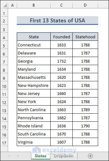
Imagine you have the following dataset in the worksheet named States. The dataset contains information about the first 13 states of the U.S.
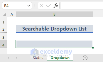
Now you want to create a searchable dropdown list in cell B4 in the worksheet named Dropdown.
Method 1 – Applying Excel Formula to Create Searchable Drop-Down List
Steps
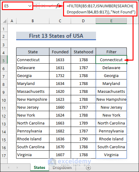
- Enter the following formula in cell E5 in the sheet named States.
=FILTER(B5:B17,ISNUMBER(SEARCH(Dropdown!B4,B5:B17)),"Not Found")The SEARCH function in the formula searches for a given value.
The ISNUMBER function returns True if the output of the Search function is a number. Otherwise, it returns False.
The FILTER function filters data according to the given criteria.
- Select cell B4 in the Dropdown worksheet.
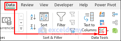
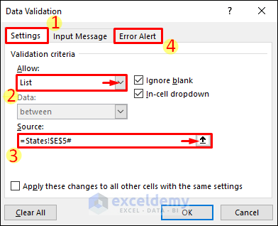
- Go to Data and choose Data Validation.
- Select the Settings tab in the Data Validation window.
- Choose List in the Allow: field using the dropdown arrow.
- Enter the following formula in the Source field.
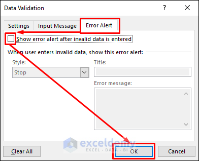
=States!$E$5#- Go to the Error Alert tab.
- Uncheck Show error alert after invalid data is entered.
- Hit the OK button.
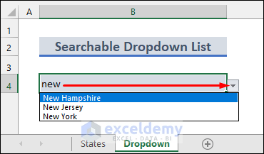
- A searchable dropdown list has been created.
- Type something in cell B4, then select the dropdown arrow visible at the lower right corner of the cell.
- You will see all the relevant search results as shown in the following picture.
Read More: How to Create Drop Down List in Multiple Columns in Excel
Method 2 – Using Excel VBA to Create Searchable Drop-Down List
Suppose we want to see the search results as shown in Google Search.
Steps
- Follow Method 1 until you reach the Data Validation steps.
- Select cell E5 in the States worksheet.
- Select Formulas and choose Name Manager.
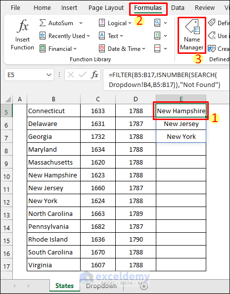
- Select New in the Name Manager window to define a list.
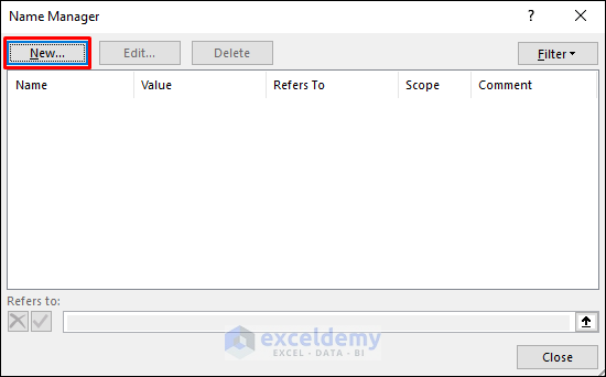
- Change the Name to Dropdown_List in the New Name window.
- Enter the following formula in the Refers to field and press OK:
=States!$E$5:$E$5:INDEX(States!$E$5:$E$17,COUNTIF(States!$E$5:$E$17,"?*"))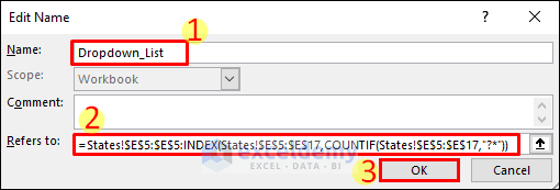
- Go to the Dropdown worksheet.
- Go to the Developer tab, and select Insert and choose Combo Box.
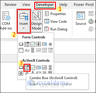
- Drag the mouse to resize the ComboBox as shown below.
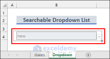
- You will see a new ComboBox created as follows.

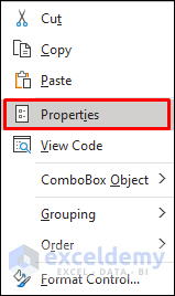
- Right-click on the ComboBox and select Properties.
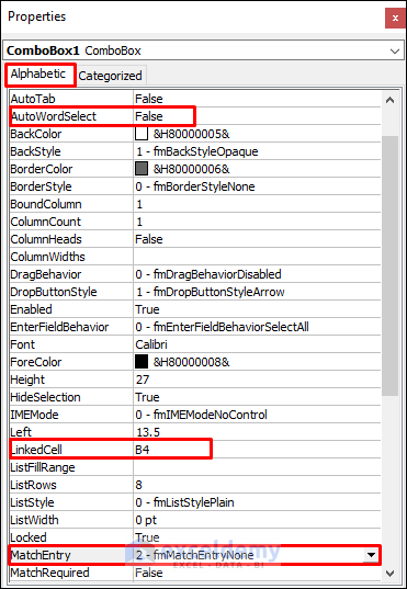
- Select the Alphabetic tab in the Properties window.
- Make the following changes: AutoWordSelect >> False, Linked Cell >> B4, MatchEntry >> 2 – fnMatchEntryNone.
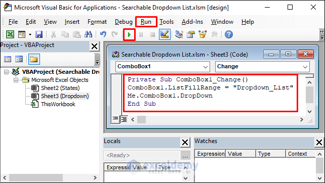
- Copy the following code:
Private Sub ComboBox1_Change()

ComboBox1.ListFillRange = "Dropdown_List"

Me.ComboBox1.DropDown

End Sub- Double-click on the ComboBox. This will take you directly to a new module in the Microsoft VBA window.
- Paste the copied code in the blank module as shown below.
- Press F5 to run the code.
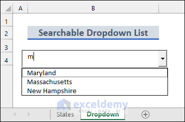
- The searchable dropdown will work like Google Search.
Things to Remember
- You need to deselect the Design Mode in the Developer tab to be able to type in the ComboBox.
- Don’t forget to make sure that the absolute references are entered properly in the formulas.
- Use Ctrl + Shift + Enter in case the array formulas are not working.
Download Practice Workbook
You can download the practice workbook from the link below.
Related Articles
- How to Add Blank Option to Drop Down List in Excel
- Creating a Drop Down Filter to Extract Data Based on Selection in Excel
- How to Select from Drop Down and Pull Data from Different Sheet in Excel
- How to Create a Form with Drop Down List in Excel
- How to Remove Used Items from Drop Down List in Excel
- How to Remove Duplicates from Drop Down List in Excel
- How to Fill Drop-Down List Cell in Excel with Color but with No Text
- [Fixed!] Drop Down List Ignore Blank Not Working in Excel
- How to Make Multiple Selection from Drop Down List in Excel
- How to Autocomplete Data Validation Drop Down List in Excel
- Hide or Unhide Columns Based on Drop Down List Selection in Excel
<< Go Back to Create Drop-Down List in Excel | Excel Drop-Down List | Data Validation in Excel | Learn Excel
Get FREE Advanced Excel Exercises with Solutions!


This was super helpful! Thank you so much, Shamim!
Glad to hear that. You are welcome!
Hi Reza,
A great article that provides a solution which works.
I have tried to set up several dropdown lists on a same sheet and the workbook seems less stable now (Excel crashes when I enter the first letters of an item in one of the search fields).
Have you had similar behaviors? Would you know how to overcome this?
Many thanks,
Chris
Hi Chris, thanks for your query.
You are facing the issue probably because the defined range is dynamic. Besides, you shouldn’t use the same defined range as the ListFillRange for multiple combo boxes. Rather you need to create a unique defined range for each of the combo boxes. You may try the following solution.
First, change the source of the defined range named as Dropdown_List to =States!$E$5:$E$17.
Then, enter the following formula in cell F5 in the States worksheet.
=FILTER(B5:B17,ISNUMBER(SEARCH(Dropdown!G4,B5:B17)),”Not Found”)
Next, create a new defined range and name it as Dropdown_List2 and enter =States!$F$5:$F$17 in the source field.
Now, insert another ComboBox in the Dropdown sheet and link it to cell G4. Enter Dropdown_List2 as the ListFillRange for this ComboBox.
After that, open the VBA window and replace the earlier code with the following one.
Private Sub ComboBox1_Change()
ComboBox1.ListFillRange = “Dropdown_List”
Me.ComboBox1.DropDown
End Sub
Private Sub ComboBox2_Change()
ComboBox2.ListFillRange = “Dropdown_List2”
Me.ComboBox2.DropDown
End Sub
Finally, run the code and hopefully you won’t face the issue again.
Thank you for the easy to follow instructions, for some reason when I follow these the search part of the drop down box doesn’t work. I am using this for a list that changes based on selection (once you select an item it is removed from the list) and that is handled in the database. The name I am using is set to a defined range, but inside that range the results change based on selections, thoughts on why the search functionality doesn’t work for me?