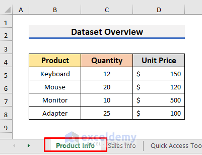
We will use two different datasets from different sheets. The first sheet contains Product Info.
The second one contains Sales Info.
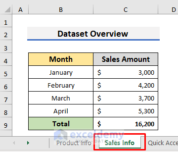
In the first method, we will create a button in Excel to navigate from the Product Info sheet to the Sales Info sheet and vice versa. We will use only the Product Info dataset in Method 2 and Method 3.
Method 1 – Use Shapes to Create a Button for Opening a Particular Sheet via Hyperlink Without Excel Macro
Steps:
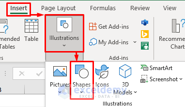
- Go to the Insert tab and click on the Illustrations icon. A drop-down menu will appear.
- Select Shapes. It will open a list of shapes.
- We selected the normal Rectangular shape.
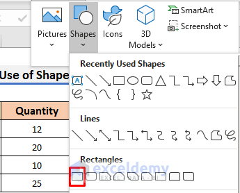
- The cursor will turn into a small black plus (+) sign.
- Click and drag the small black plus (+) symbol to draw a rectangular shape like the picture below.
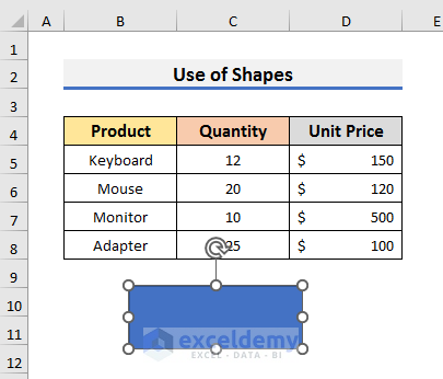
- Type a name on it and change the font size if you want.
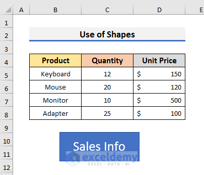
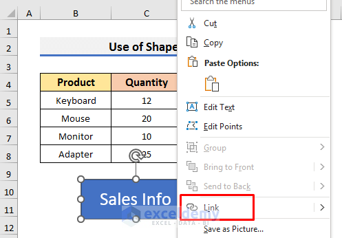
- Right–click on the Sales Info button and select Link from the menu. The Insert Hyperlink window will appear.
- In the Insert Hyperlink box, select the Place In This Document option and choose the sheet name. We have selected Sales Info.
- Click OK to proceed.
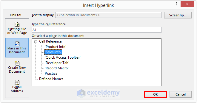
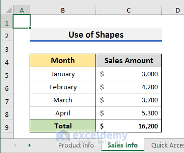
Note: When you click on the button, it will take you to the Cell A1 of the Sales Info sheet. You can change the cell in the “Type the cell reference” field. If you want to go to Cell B5 of a sheet, type B5 in that field.
- This creates a button on the desired sheet.
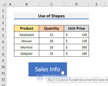
- If you click on the Sales Info button, it will take you to the Sales Info sheet.
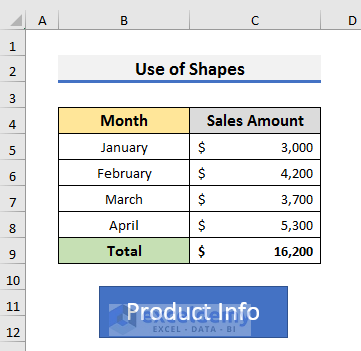
- You can also create the Product Info button to move to the Product Info sheet.
Read More: Excel Hyperlink with Shortcut Key
Method 2 – Create a Button Without Macro from the Quick Access Toolbar
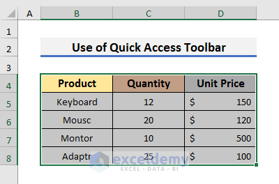
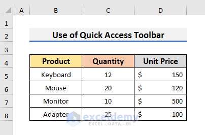
In the dataset below, there are 3 misspelled words. We will add a button to the Quick Access Toolbar to perform a spell check with one click.
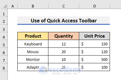
Steps:
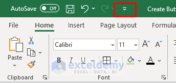
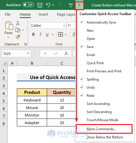
- Click on the Customize Quick Access Toolbar icon. A drop-down menu will appear.
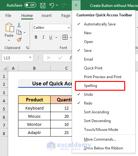
- Select Spelling from the drop-down menu.
- You can choose other options to perform other tasks. To see the Print Preview with a single click, you can add the “Print Preview and Print” button.
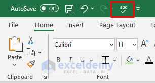
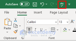
- You will get the Spelling button on the toolbar.
- Select the range B4:D8.
- Click on the Spelling button.
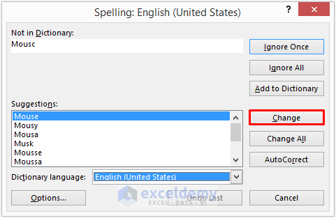
- You will get the Spelling box.
- Select the desired spelling from the Suggestions section and click on the Change option to apply the new spelling.
- You will get results like the screenshot below.
Note: To find more functions:
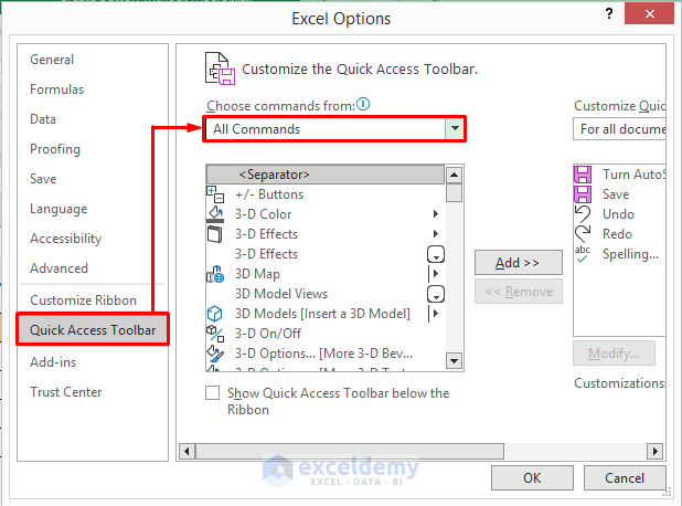
- Click on the More Commands option.
- Select All Commands from the “Choose commands from” section.
- You can add other buttons from here.
Read More: How to Create Button to Link to Another Sheet in Excel
Method 3 – Add a Button from the Developer Tab Without Macro in Excel
We will add a Scroll Button in Column D to set the quantity of the products.
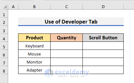
Steps:
- Go to the Developer tab and select Insert. A drop-down menu will appear.
- Select Scroll Button from the “Form Controls” section.
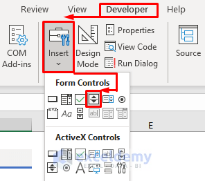
- Draw the button in Cell D5.
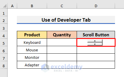
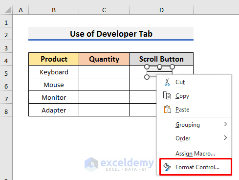
- Right–click on the button to open the menu.
- Select Format Control from there.
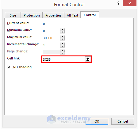
- In the Format Control box, set the cell that you want to link in the Cell link field.
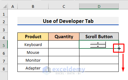
- Drag the Fill Handle down to copy the Scroll Button in the below cells.
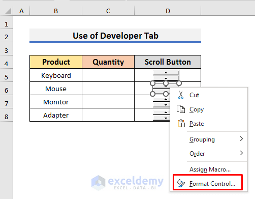
- Format each Scroll Button individually and link the desired cells.
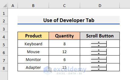
- Click on the Scroll Button to set the quantity of the products.
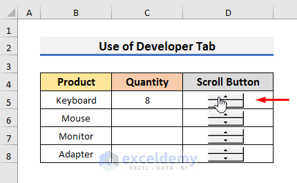
- You will see the results like the picture below after.
How to Create a Button with Record Macro in Excel
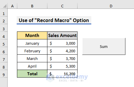
We will use a dataset that contains the sum of the sales for the first four months. We will assign a macro in the button to calculate the sum of the range C5:C8 automatically.
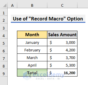
Steps:
- Go to the Developer tab and click on the Insert icon. It will open a drop-down menu.
- Select the Button icon from the Form Controls section.
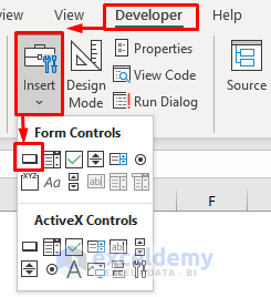
- The cursor will change into a small black plus (+) symbol.
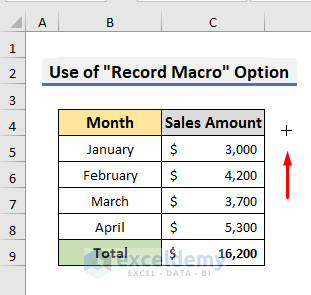
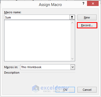
- Click and drag the small black plus (+) icon to draw the button. The Assign Macro box will appear.
- Change the Macro name and select Record from there.
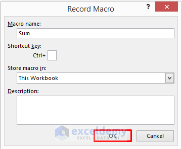
- Another box will appear with default values. Click OK to proceed.
- Right–click on the button and set its name.
- Remove the contents of Cell C9 and insert the formula below:
=SUM(C5:C8)- Press Enter to see the result.
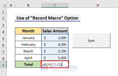
We have used the SUM function to calculate the sum of the range C5:C8.
- Navigate to the Developer tab and select Stop Recording from there.

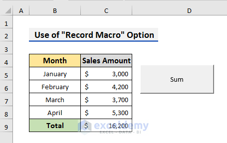
- If the Cell C9 is blank, click on the Sum Button.
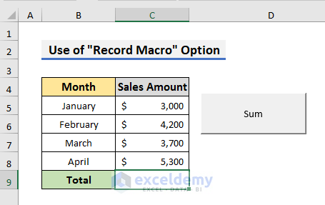
- You will see the sum with a single click on the button.
Read More: How to Convert Text to Hyperlink in Excel
Download the Practice Workbook
Related Articles
- How to Hyperlink Multiple Cells in Excel
- How to Activate Multiple Hyperlinks in Excel
- How to Fix Broken Hyperlinks in Excel
- How to Hyperlink to Cell in Excel
- How to Hyperlink Multiple PDF Files in Excel
- How to Link Files in Excel
<< Go Back To Hyperlink in Excel | Linking in Excel | Learn Excel
Get FREE Advanced Excel Exercises with Solutions!

