How to Create a Date Hierarchy in an Excel Pivot Table – 7 Steps

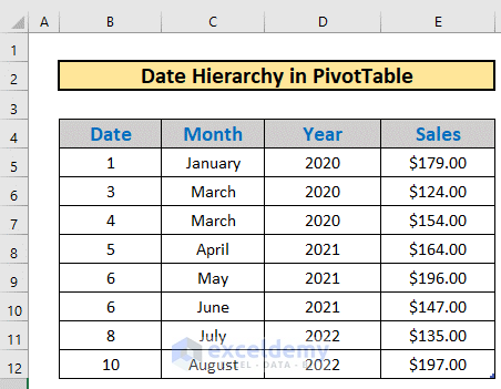
This is the sample dataset.

Step 1 – Add the Dataset to the Data Model

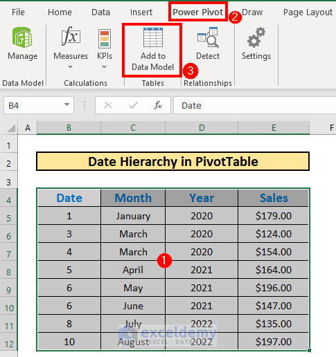
• Select the entire dataset B4:E12.
• Go to Power Pivot
• Select Add to Data Model.

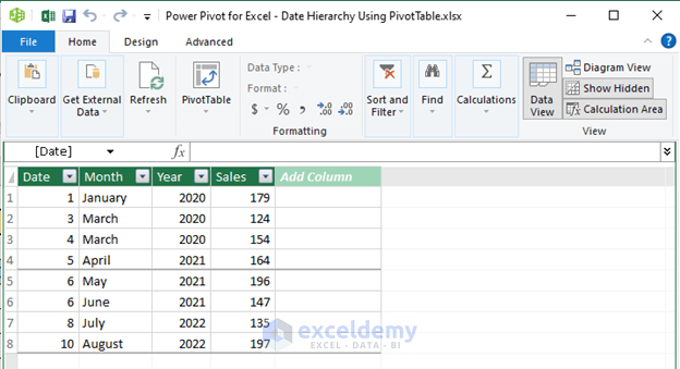
• Excel will add the dataset to the data model.

Step 2 – Activate the Diagram View

• Select Diagram View in Data Model

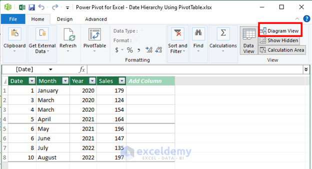
• Excel will activate the Diagram View.

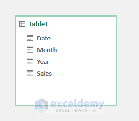
Step 3 – Select the Columns to Create a Hierarchy

• Select the column Year.
• Right-click .
• Select Create Hierarchy.

• Excel will create a hierarchy.
• Rename it. Here, Date Hierarchy.

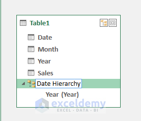
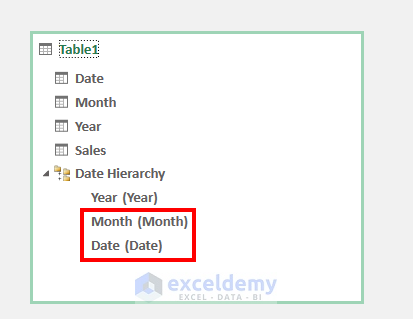
Step 4 –  Create a Child Hierarchy Level

The Month and Date columns will be the child levels:

• Drag them one by one within the parent hierarchy level.

Read More: How to Create Multi Level Hierarchy in Excel

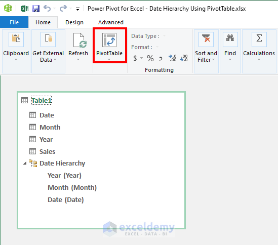
Step 5 – Create a PivotTable

• Select PivotTable.

• Select New Worksheet.
• Click OK.

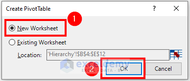
• Excel will create a PivotTable.

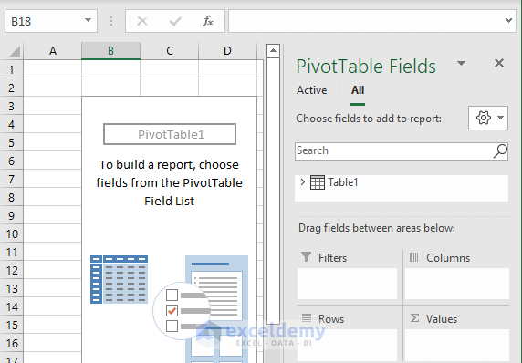
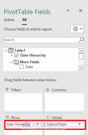
Step 6 – Edit the PivotTable Fields

• Drag Date Hierarchy to Rows and Sales to Values. You will find the Sales column in More Fields

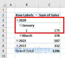
• To see the hierarchy, click the + icon.

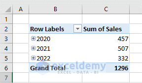
This is the output.

Read More: How to Add Row Hierarchy in Excel

Step 7 – Format the PivotTable

Read More: How to Create Hierarchy in Excel Pivot Table

Things to Remember

• You must activate the Power Pivot add-in.

Download Practice Workbook

Download this dataset and practice.

Related Articles

• How to Make Hierarchy Chart in Excel
  
• How to Use SmartArt Hierarchy in Excel
• How to Create a Hierarchy of the State City and Zip Code in Excel

<< Go Back to Hierarchy in Excel | SmartArt in Excel | Learn Excel