Dividend Reinvestment Formulas
Inputs:
- Initial Balance: This is the balance you have at the beginning of your calculation of dividend reinvestment.
- Dividend Data: This is the dividend that you get from the stock market or business every month, quarter, or year.
- Stock/Share Price: Stock price or business’s share price at the beginning and end of a month, quarter, or year.
Outputs:
- Shares Beginning: This is the number of shares that you have at the beginning of the calculation.
For the first month:
Shares Beginning = (Initial Balance/Share price at the beginning of the month)
For all the next months:
Shares Beginning = (Shares Beginning at the previous month + Reinvestment of the previous month)
- Reinvestment: This is the number of shares that you reinvested through your dividends.
Reinvestment = [(Dividend×Shares Beginning)/Share price at the end of the month]
- Ending Reinvest Balance: Thighs is the ending balance of your principal after reinvesting your dividends.
Ending Reinvest Balance = [(Shares Beginning+Reinvestment)×Share price at the end of the month]
- Ending Balance: This is the last ending reinvestment balance of your calculation.
- Cumulative Return: This is the cumulative return for reinvesting the dividends.
Cumulative Return = [(Initial Investment/Ending Balance) -1]×100%
How to Create a Dividend Reinvestment Calculator with Monthly Contributions in Excel: with Easy Steps
Step 1 – Record Dividend Data
- Create a worksheet named the Dividend Database.
- Record the dividend data.
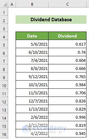
- As the data is in irregular dates, you will need to extract the month and year. Insert a column between Date and Dividend columns named Month & Year.

- Click on the C5 cell and insert the formula below, then press the Enter button.
=TEXT(B5,"mmyy")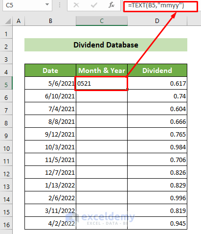
- Place your cursor in the bottom-right corner of the cell. When the fill handle appears, drag it down to copy the formula for all other dates.
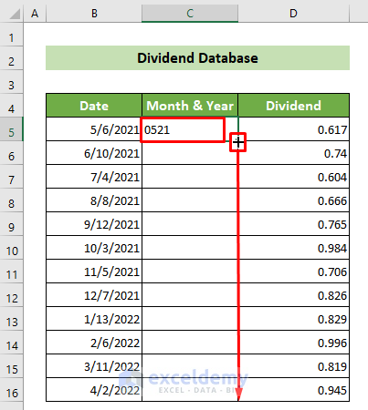
You will get an organized dividend dataset.
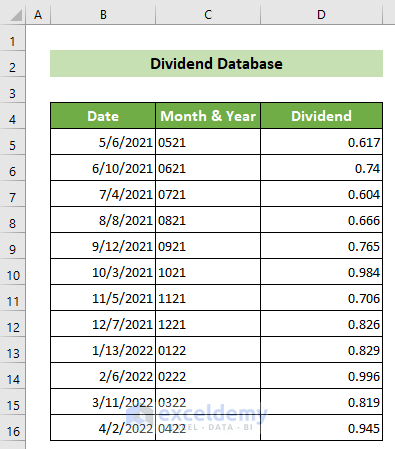
Step 2 – Organize the Share Prices and Dividends
- Record the starting date of every month along with the share price at the beginning and the end of the month.
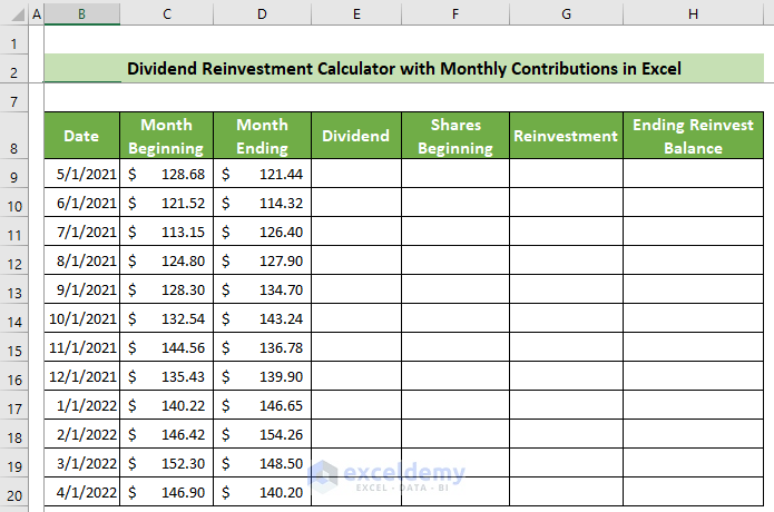
- You need to find the dividend for each following month. Click on the E9 cell and insert the following formula, then press the Enter button.
=VLOOKUP(TEXT(B9,"mmyy"),'Dividend Database'!$C$5:$D$16,2,FALSE)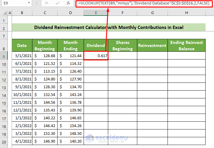
Formula Explanation:
- TEXT(B9,”mmyy”)
This returns the value of the B9 cell’s date in text format with the date’s month and year.
Result: 0521
- =VLOOKUP(TEXT(B9,”mmyy”),’Dividend Database’!$C$5:$D$16,2,FALSE)
This looks up the previous result in the Dividend Database worksheet’s C5:D16 range and returns the 2nd column value where the lookup value is found.
Result: 0.617
Notes:
- The data range should be made absolute to avoid errors. You can do this by putting a Dollar sign ($) or else you can simply press the F4 key.
- The column containing the lookup value should be the first column of the table array as you have used the VLOOKUP function. Otherwise, errors will occur.
- Place your cursor on the bottom-right position of your cell, and the Fill Handle will appear. Drag it down to copy the formula for all the other cells below.
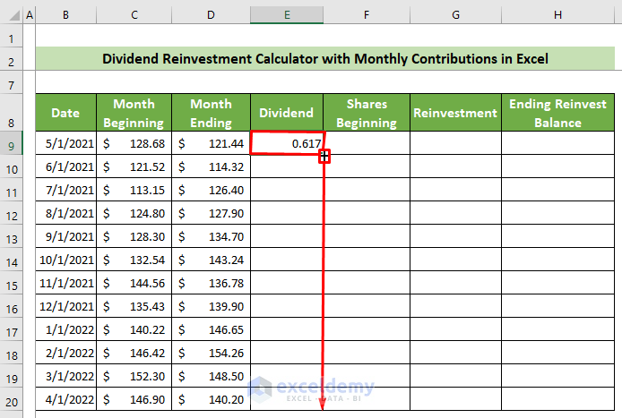
The outcome should look like this.
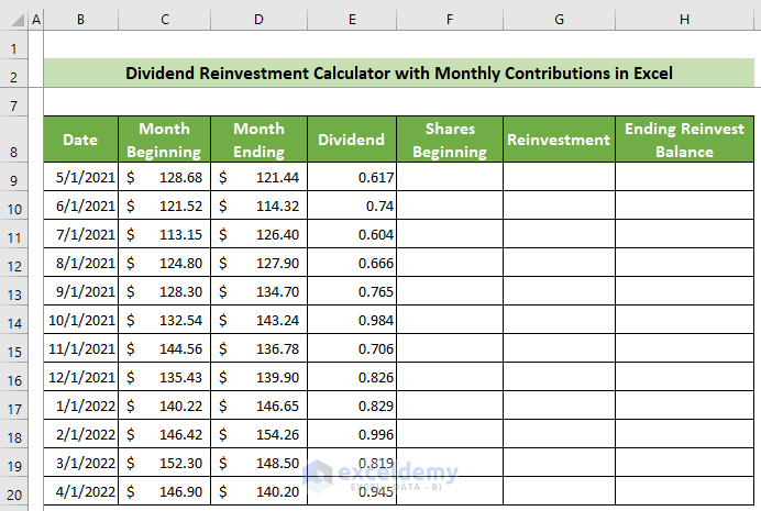
Step 3 – Calculate the Monthly Dividend Reinvestment
- Put your initial investment at the F4 cell of the sheet.

- Click on the F9 cell and use the following formula to calculate the number of shares at the beginning of your investment.
=F4/C9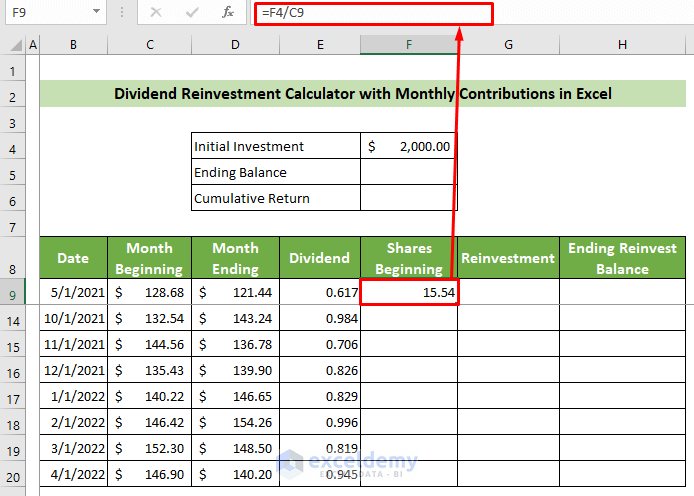
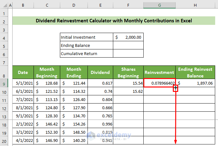
- Click on the G9 cell and use the following formula to find the reinvestment for the following month.
=E9*F9/D9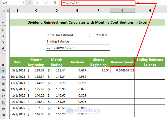
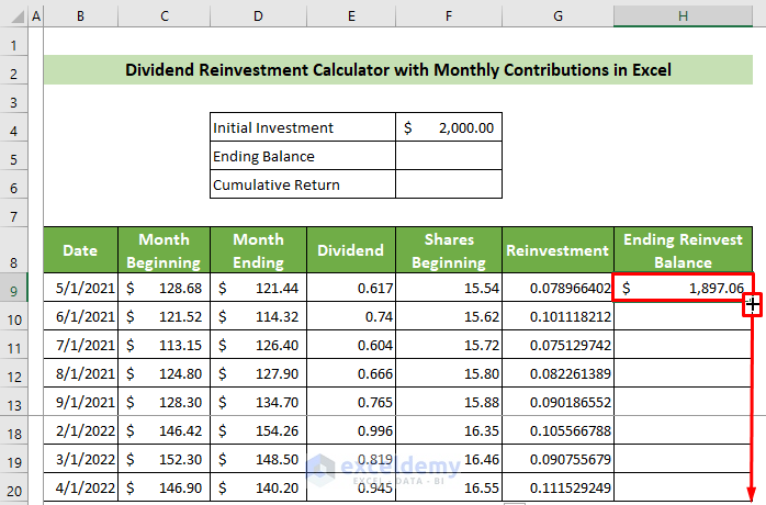
- Click on the H9 cell and insert the following formula, then press the Enter button.
=SUM(F9,G9)*D9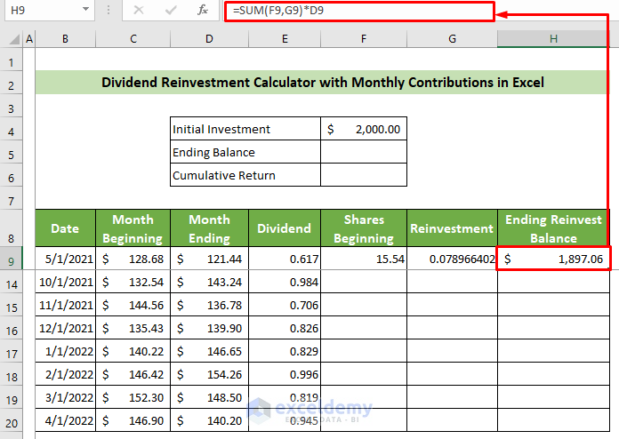
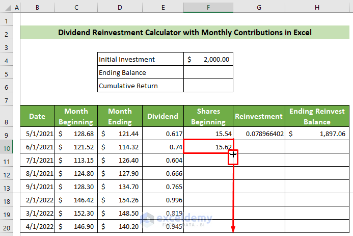
- For calculating the second month’s shares beginning, insert the following formula at the F10 cell and press the Enter button.
=SUM(F9,G9)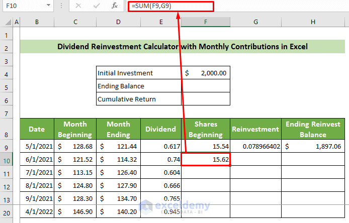
- Drag the F9 cell’s Fill Handle down.
- Repeat the filling for G9.
- Fill the H column as well.
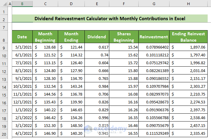
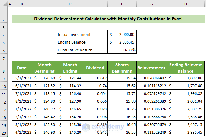
Here’s the resulting table.
Step 4 – Calculate the Return of Reinvestment
- Click on the F5 cell and refer to the H20 cell’s value.

- Click on the F6 cell and insert the formula below.
=F5/F4-1- Press the Enter button.
- Make this cell’s number format as Percentage.

Here’s the result.
Download the Sample Workbook
Related Articles
- How to Create Mortgage Loan Pipeline Management in Excel
- How to Create Fibonacci Calculator in Excel
- How to Create a Fibonacci Pivot Point Calculator in Excel
<< Go Back to Finance Template | Excel Templates
Get FREE Advanced Excel Exercises with Solutions!

