The sample dataset showcases Unit Cost vs Produced Unit. 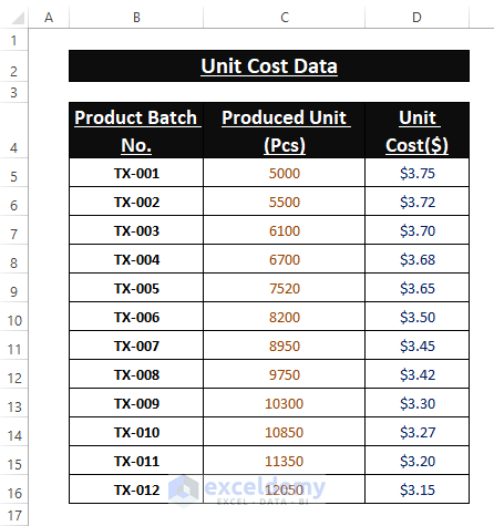
What Is Linear Regression?
Regression Analysis deals with predicting values that depend on two or more variables. Linear Regression estimates values with single dependent and independent variables. The equation is : Y=mX+C+E and the variables are:
Y = Dependent Variable
m = Slope of the Regression Formula
X = Independent Variable
Ε = Error Term, the difference between the actual value and predicted value.
The error term, E is in the formula because no prediction is 100% correct.
The Linear Regression formula becomes: Y=mX+C, if the error term is ignored.
Method 1 – Performing Simple Linear Regression Using the Analysis Toolpak in Excel
- Go to File > Options.

Step 2:
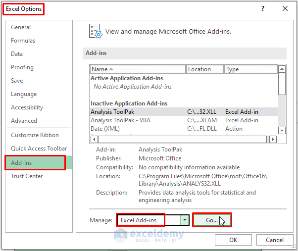
- Select Add-ins > Choose Excel Add-ins in Manage > Click Go.
Step 3:
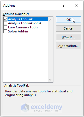
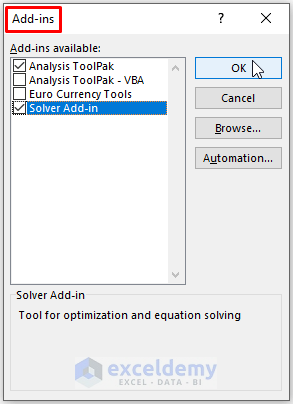
- In the Add-ins window, check Analysis Toolpak > Click OK.
Step 4:
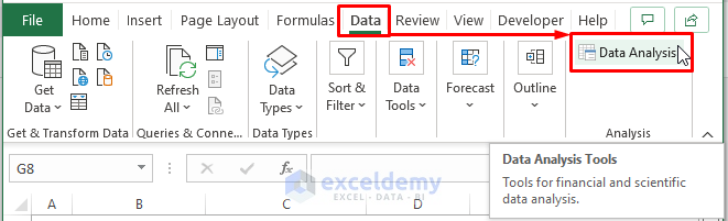
- Go back to the worksheet and select Data > Data Analysis.
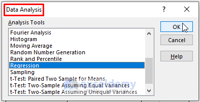
Step 5:
- Select Regression in Analysis Tools and click OK.
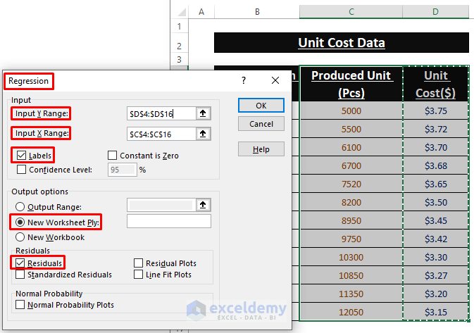
Step 6:
- In the Regression dialog box, assign cell values to Input Y (Column D) and X (Column C) Ranges.
Linear Regression Analysis Outcome
1. Regression Statistics:
Regression Statistics is an array of different parameters that indicate how well the measured Linear Regression describes the data model.
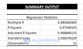
Multiple R: indicates a correlation between variables. Its value ranges from -1 to 1. The more positive the value, the stronger the correlative relationships:
1: a strong positive relationship.
-1: a strong negative relationship.
0: no relationship.
R Square: the Coefficient of Determination. It indicates how well the data model fits the Regression Analysis. It also depicts the number of points that fall on the Regression Equation Line. It is calculated using the Total Sum of Squares. The R2 value is 0.9714.., so 97.14% of the data value falls in the Regression model and the same percentages of dependent variables are relatable by independent variables. An R2 value of more than 95% is taken as a good fit.
Adjusted R Square: The adjusted value of R2 is used in multiple variables Regression Analysis.
Standard Error: The smaller the Standard Error, the more accurate the Linear Regression equation. It shows the average distance of data points in the Linear equation.
Observations: The iteration number of the data model.
2. ANOVA Outcome
It’s the variance analysis that displays the variability of a data model.
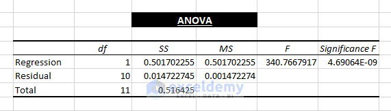
ANOVA divides the Sum of Squares portion into parameters that provide information on the shifting within the Regression Analysis. The parameters are:
df: the number of degrees of freedom (nDOF) related to the variance sources.
SS: Sum of Squares; SS is considered the good to fit parameter. The less the Residual value of SS, the better it fits the the Total SS value.
MS: The Mean Square is known as MS.
F: F statistic or F-test refers to the Null Hypothesis. It tests the overall significance of the regression model.
Significance F: The P-Value of F.
The ANOVA calculation is less important than conducting a Linear Regression Analysis. However, the Significance F parameter is important. A Significance F value less than 5% or 0.05 indicates the a good fit to the data model.
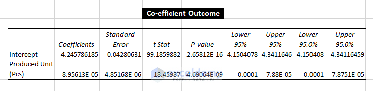
3. Co-efficient Outcome:
The coefficients are used to calculate Y values.
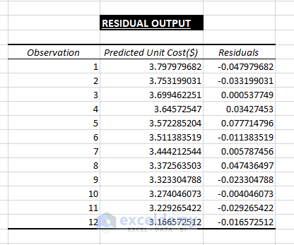
4. Residual Output:
It compares the calculated values with the estimated values as depicted below.
Read More: Multiple Linear Regression on Excel Data Sets
Method 2 – Displaying a Linear Regression Equation in an Excel Chart
Step 1:
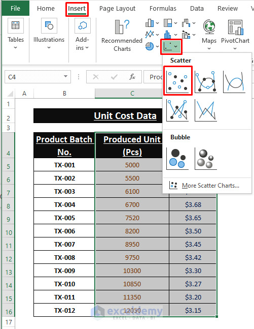
- Select the columns (C and D).
- Go to Insert > Click Scatter (in Charts).
Step 2:
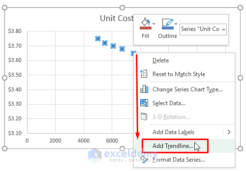
Excel immediately inserts the Chart with scatter points.
- Right-click one of the points.
- Select Add Trendline.
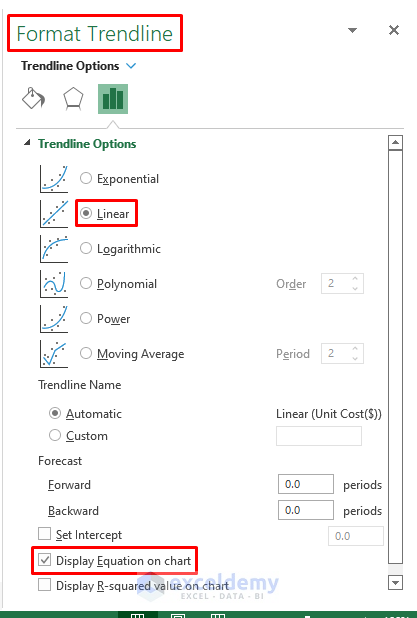
Step 3:
- In the Format Trendline window, check Linear and Display Equation on Chart.
Step 4:
- Use the Chart Element feature to complete the Chart as shown below.
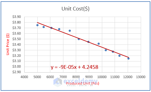
You will see the Linear Regression equation and the m and C values.
Method 3: Performing Linear Regression Using Multiple Functions in Excel
- Enter the following formula in F6.
=LINEST(D5:D16,C5:C16)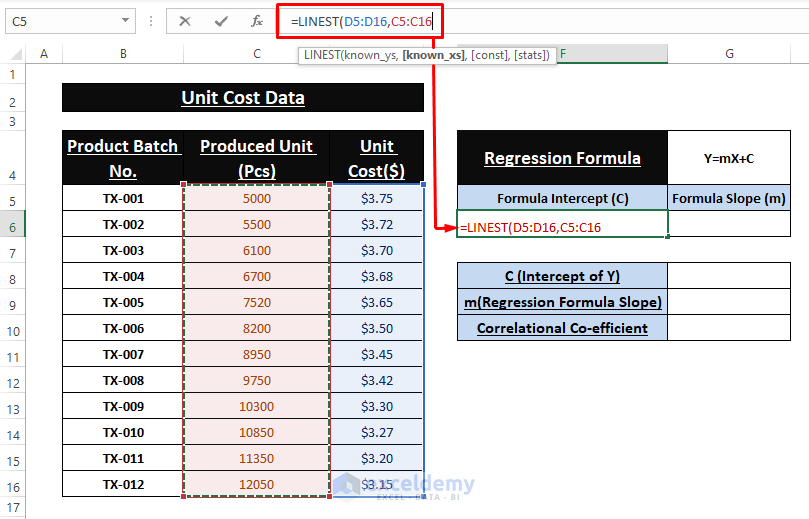
- As it’s an array formula, press CTRL+SHIFT+ENTER.
The INTERCEPT Function:
- Enter the equation in G8 to find the value.
=INTERCEPT(D5:D16,C5:C16)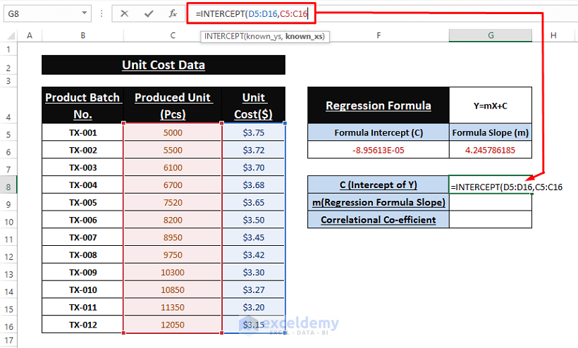
- Use the formula below to calculate the slope.
=SLOPE(D5:D16,C5:C16)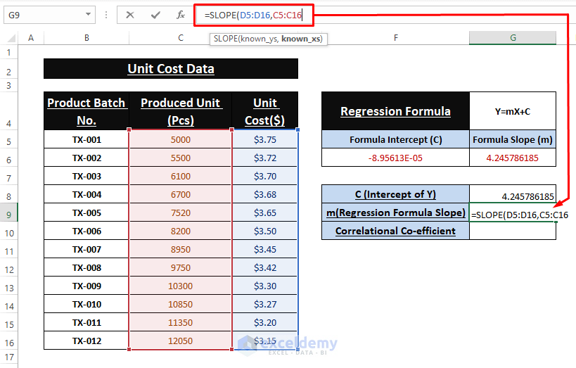
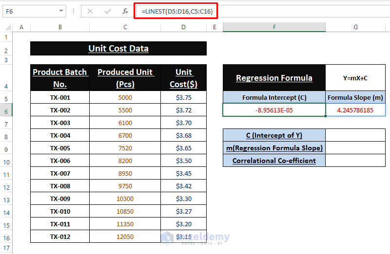
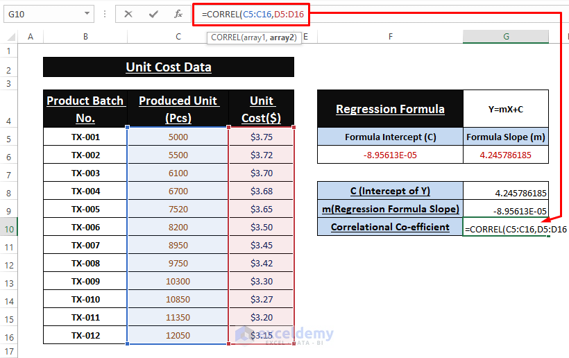
Find an additional parameter to depict how strongly the two variables are connected.
- Enter the following formula in G10.
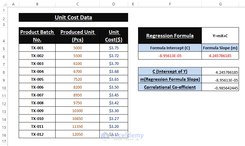
The image below displays the outputs of the used formulas:
Read More:
Method 4 – Using the Solver Add-in to Trial-Error Test Linear Regression Outcomes
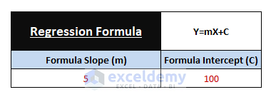
1. Using Assumed Values for Slope (m) and Intercept (C):
- Input values as Slope (here, 5) and Intercept (here., 75).
2. Calculating Y Values:
- Use the formula below.
=$G$4*B3+$H$4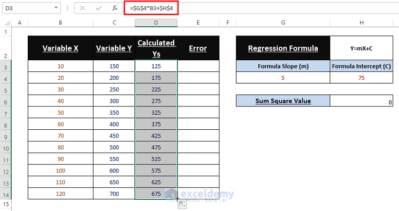
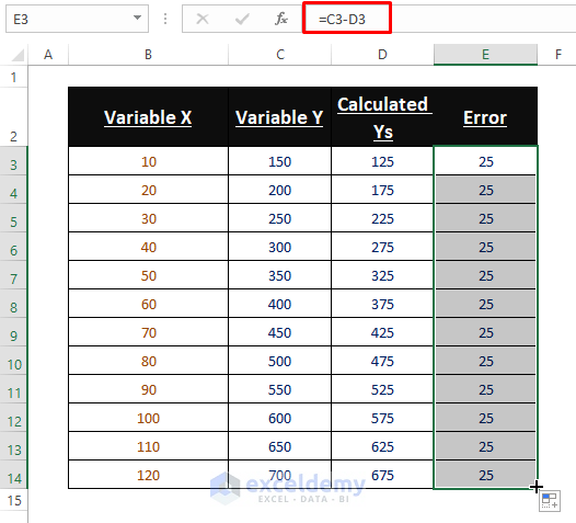
3. Error Amounts between Y Values:
- Execute an Arithmetic Operation (Subtraction) to find error amounts in Y values.
Find the Sum of Squares in the error column. Here, the SUMSQ function is used as a tool in the Solver Add-in to minimize the error.
- Use the following formula in H6.
=SUMSQ(E3:E14)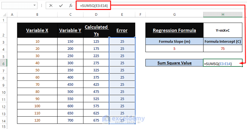
4. Using the Solver Add-in:
- Enable the Solver Add-in following the steps described in Method 1.
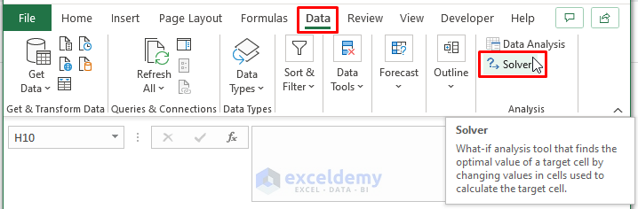
- Go to Data > Click Solver (in Analysis).
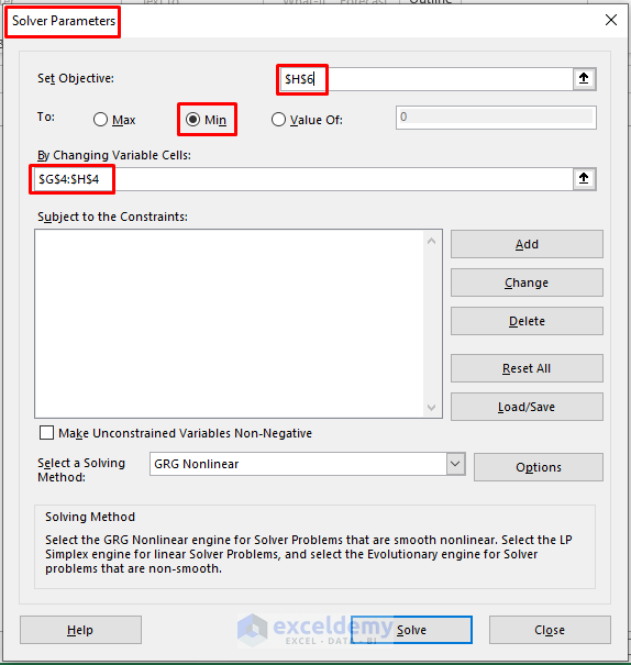
In the Solve Parameters dialog box:
- Assign Set Objective as H6 (the Sum of Square value).
- Select Min in To.
- Enter Slope (m) and Intercept (C) variable values in By Changing Variable Cells.
- Click Solve.
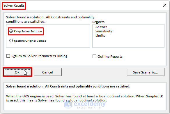
- In the Solver Results window, select Keep Solver Solution.
- Click OK.
Download Excel Workbook
Related Articles
- How to Do Logistic Regression in Excel
- How to Do Multiple Regression Analysis in Excel
- Calculate P Value in Linear Regression in Excel
- How to Interpret Multiple Regression Results in Excel
- How to Interpret Linear Regression Results in Excel
- How to Plot Least Squares Regression Line in Excel
<< Go Back to Regression Analysis in Excel | Excel for Statistics | Learn Excel
Get FREE Advanced Excel Exercises with Solutions!
