Looking for a way to format a double column cash book in Excel? Then, this is the right place for you. Here, you will find a step-by-step different way to format a double column cash book in Excel.
What Is Cash Book?
Cash Book is a kind of ledger account that records regular cash and bank transactions in chronological order of a company. There are 4 types of Cash Books.
1. Single Column
2. Double Column with Discount
3. Double Column with Tax
4. Triple Column with Discount and Tax
What Is Double Column Cash Book?
Double Column Cash Book is used to record cash and bank transactions with two columns on each side. It is also known as two column cash book.
How to Format Double Column Cash Book in Excel: Step by Step Procedures
Here, we will show you how you can format a double column cash book in Excel by going through the following 8 steps.
Step 1: Insert Headers
In the first step, you will have to insert headers to create a double column cash book and then format them in Excel.
To do that, follow the steps given below.
Steps:
- To begin with, type Serial No, Date, Description, Cash and Bank to create headers.
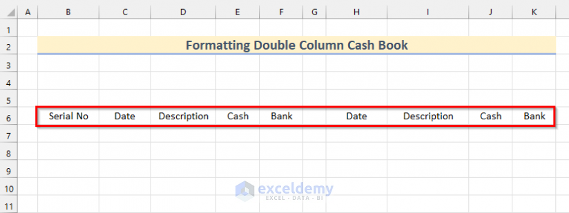
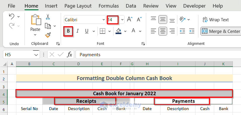
- Then, select cell range C5:F5 and click on Merge & Center from the Home tab.

- Now, type Receipts as a header.

- Similarly, merge & center cell range H5:K5 and type Payments.

- Again, add another header as Cash Book for January 2022 by merging & centering cell range B4:K4.

- After that, select the 3 headers below pressing Ctrl on your keyboard.
- Next, click on the Bold button and set 14 as the Font Size from the Home tab.
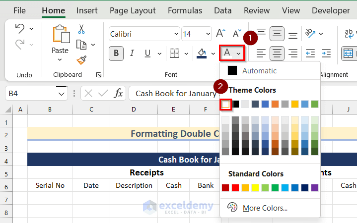
- Further, select the header Cash Book for January 2022 and click on Fill Color from the Home tab.

- Now, select any color of your own choice. Here, we will select Blue, Accent 1, Darker 50%.

- Click on Font Color and select any color of your choice. Here, we will select White, Background 1.
- Similarly, you can format the other headers according to your wish.

Step 2: Create Table to Format in Excel
Next, we will create a table to format a double column cash book in Excel. Go through the steps given below to do it on your own.
Steps:
- Firstly, select cell range B6:K7.
- Secondly, go to the Home tab >> click on Borders.
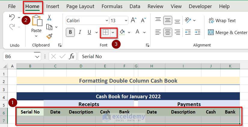
- Then, select All Borders.

- After that, press the keyboard shortcut Ctrl + T to create a table.

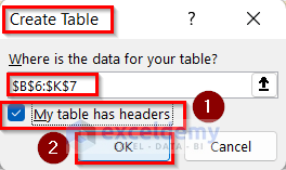
- Now, the Create Table box will open.
- Here, you will see that the cell range has already been selected.
- Afterward, turn on My table has header option.
- Finally, click on OK.
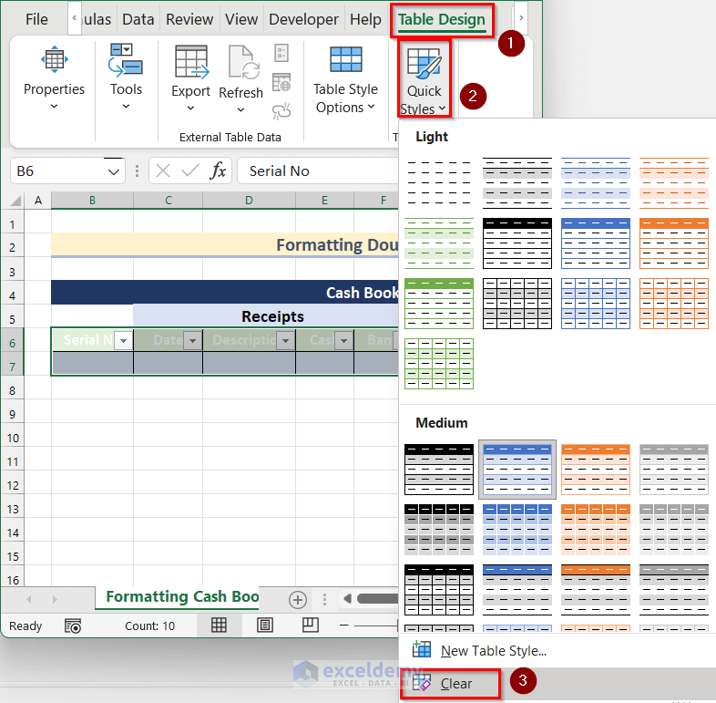
- Next, go to the Table Design tab >> click on Quick Style >> select Clear.
- Further, press Ctrl + Shift +L.
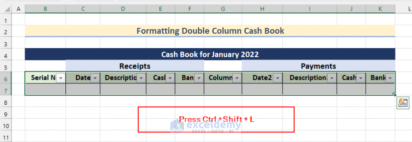
- Thus, a table will be created.

- Here, to remove the header in Cell G6, select the Cell.

- After selecting, remove the text by pressing Backspace using your keyboard.
- In the end, insert a space and then press Enter.

- Similarly, you can edit the other headers by inserting a space and then pressing Enter.

Read More: How to Create Petty Cash Book Format in Excel
Step 3: Use IF & ROWS Functions to Update Serial Number
Now, we will show you how you can update the serial number using the IF and ROWS function in Excel to format a double column cash book.
Steps:
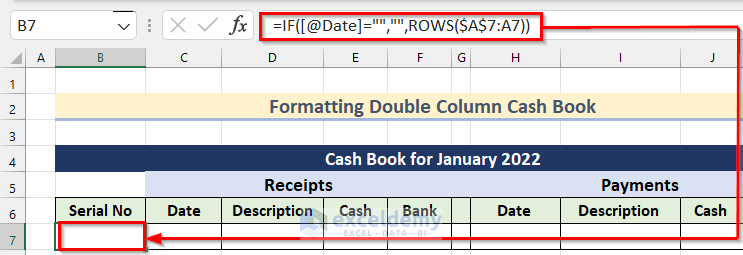
- In the beginning, select Cell B7 and insert the following formula.
=IF([@Date]="","",ROWS($A$7:A7))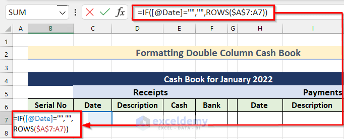
- Then, press Enter.
🔎 How does the Formula Work?
- ROWS($A$7:A7)—–> The ROWS function returns the count value of the rows given in the function.
Output: {1}
- IF([@Date]=””,””,ROWS($A$7:A7))—–> The IF function returns a value if the given condition is TRUE and returns a different value if the condition is FALSE.
IF([@Date]=””,””,1)—–> turns into
Output: {1}
- Now, if you insert a date in the Date column the Serial No will automatically get updated.

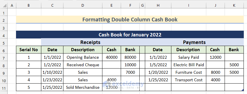
Step 4: Enter Data into Double Column Cash Book
Next, enter your data into the double column cash book you have prepared till now.
Step 5: Change Number Format to Format Double Column Cash Book
In the fifth step, we will show you how you can change the Number Format in Excel to format a double column cash book.
Steps:
- Firstly, select the cell ranges which need a change in the Number Format. Here, we will select cell ranges E7:F11 and J7:K11 to change the Number Format to Currency.
- After that, go to the Home tab >> click on Number >> click on Number Format.
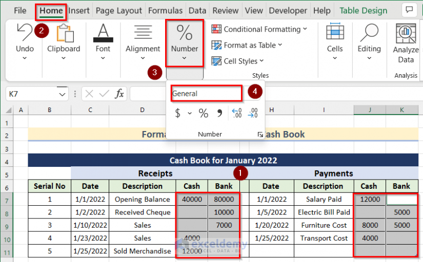
- Next, select Currency.

- Thus, you can change Number Format in Excel.

Step 6: Calculate Total Cash & Bank for Receipts in Cash Book in Excel
Now, we will show you how to calculate Total Cash and Bank for Receipts in a double column cash book.

Go through the steps given below to do it on your own.
Steps:
- In the beginning, select Cell N6 and insert the following formula.
=SUM(Table4[Cash])
- Next, press Enter and get the value of Total Cash for Receipts.

- After that, select Cell N7 and insert the following formula.
=SUM(Table4[Bank])
- Then, press Enter.

- Now, select Cell N8 and insert the following formula.
=SUM(N6:N7)
- Finally, press Enter.

- Now, if you add, edit or delete any data in the table for Receipts, the resultant values for Receipts will automatically update.
Step 7: Determine Total Cash and Bank & Payments in Double Column Cash Book
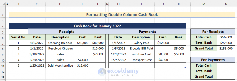
Similarly, you can determine the Total Cash and Bank for payments in a double column cash book following the steps given below.
Steps:
- Firstly, select Cell N11 and insert the following formula.
=SUM(Table4[[Cash ]])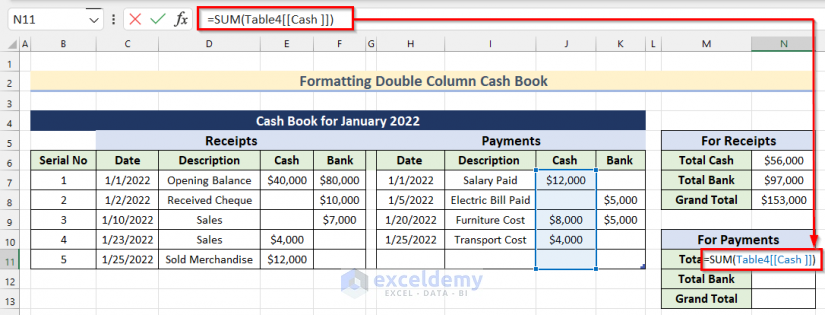
- Then, press Enter.

- Secondly, select Cell N12 and insert the following formula.
=SUM(Table4[[Bank ]])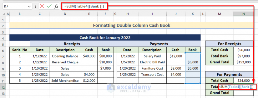
- Now, press Enter to get the value of Total Bank amount for Payments.

- After that, select Cell N12 and insert the following formula.
=SUM(N11:N12)
- Finally, press Enter to get the value of Grand Total for Payments.
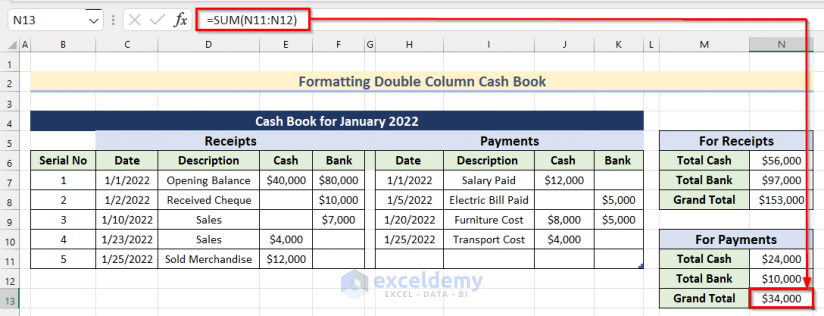
- Next, if you add, edit or delete any data in the table for Payments, the resultant values for Payments will automatically update.
Step 8: Figure Out Closing Balance of Cash Book in Excel
In the last step, we will figure out the Closing Balance of a double column cash book in Excel.
Steps:
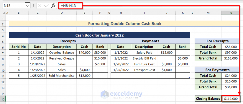
- To start with, select Cell N15 and insert the formula given below.
=N8-N13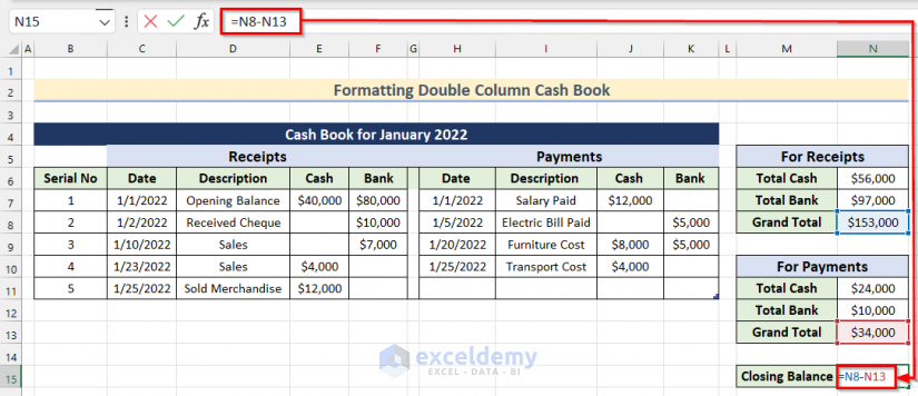
- Then, press Enter and get the value of Closing Balance.
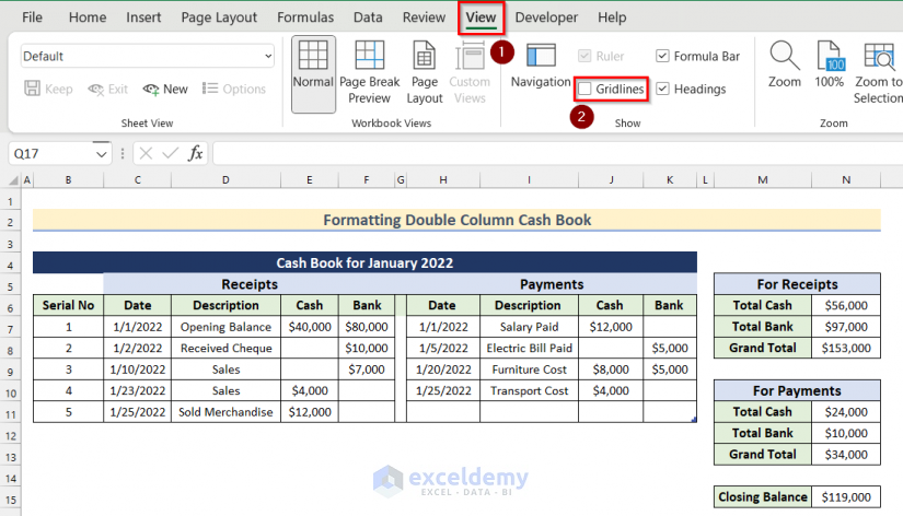
Now, to get a clear vision of the cask book you can turn off the Gridlines from your Excel worksheet.
- To do that, go to the View tab >> turn off Gridlines.
- That’s it!! Thus, you can format a double column cash book in Excel.
- Now, if you add, edit or delete any data in the table the whole dataset will change accordingly.

Things to Remember
- All the Cash and Bank received are considered Debits and payments are Credits.
- Closing Balance is figured out after a specific period of time calculating both total cash and bank amounts for receipts and payments.
Download Practice Workbook
You can download the workbook to practice yourself.
Conclusion
So, in this article, we have shown you ways to format a double column cash book in Excel. I hope you found this article interesting and helpful. If something seems difficult to understand, please leave a comment. Please let us know if there are any more alternatives that we may have missed. Thank you!
Related Articles
<< Go Back to Excel Cash Book Templates | Accounting Templates | Excel Templates
Get FREE Advanced Excel Exercises with Solutions!

