The dataset showcases sports Event(s) and the List of Winners.
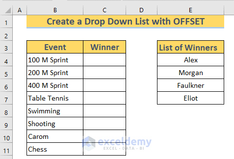
Method 1 – Create a Dynamic Drop Down List with the OFFSET and the COUNTA Functions
STEPS:
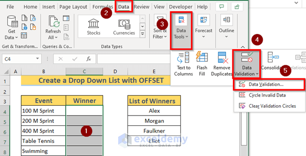
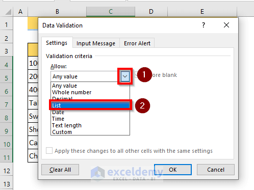
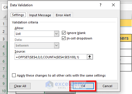
- In the Data Validation dialog box, select List.
- In Source, enter the following formula.
=OFFSET($E$4,0,0,COUNTA($E$4:$E$100),1)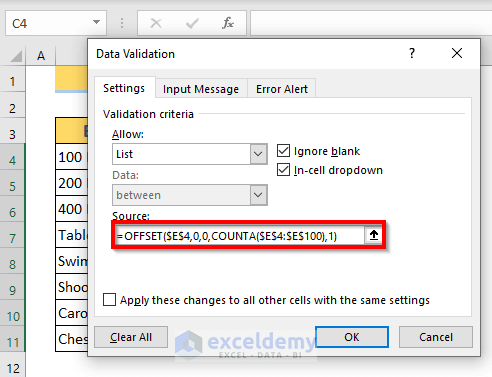
Formula Breakdown
➥ COUNTA($E$4:$E$100) ➜ Returns the number of cells that are not empty in E4:E100
Output ➜ {4}
➥ OFFSET($E$4,0,0,COUNTA($E$4:$E$100),1) ➜ Returns a range based on the row and column of a given reference.
➥ OFFSET($E$4,0,0,4,1)
Output ➜ {“Alex”;”Morgan”;”Faulkner”;”Eliot”}
Explanation: The reference is E4. Since the row is 0 and the column is 0 with a height of 4 cells, the function returns the values in E4:E7.
- Click OK.
Excel will create a drop-down box in each cell in C4:C11.
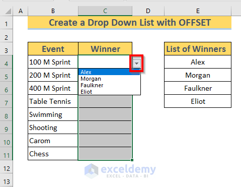
The options in the drop-down box are the names in the List of Winners.
To check whether this is a dynamic drop-down box, assume that the Winner of Shooting is James. Since James is not in the List of Winners, add his name.
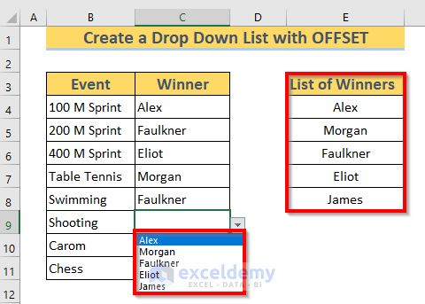
Excel automatically updated the drop-down options.
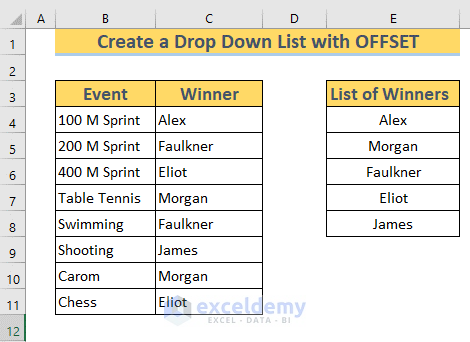
NOTE: The selected range in the COUNTA Function is E4:E100. Excel will update the drop-down options if you add or update data in E4:E100.
Method 2 – Create a Dynamic Drop Down List in Excel with the OFFSET and COUNTIF Functions
STEPS:
- Go to Data Validation ( as described in method-1).
- In Source, use the following formula
=OFFSET($E$4,0,0,COUNTIF($E$4:$E$100,"<>"))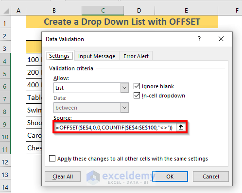
Formula Breakdown
➥ COUNTIF($E$4:$E$100,”<>”)➜ Returns the number of cells that are not empty in E4:E100
Output ➜ {4}
➥ OFFSET($E$4,0,0,COUNTIF($E$4:$E$100,”<>”)) ➜ Returns a range based on the row and column of a given reference.
➥ OFFSET($E$4,0,0,4,1)
Output ➜ {“Alex”;”Morgan”;”Faulkner”;”Eliot”}
Explanation: The reference is E4. Since the row is 0 and the column is 0 with a height of 4 cells, the function returns the values in E4:E7
- Cilck OK.
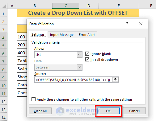
- Excel will create a drop-down box in each cell in C4:C11.

To check whether this is a dynamic drop-down box, assume the Winner of Shooting is James. Since James is not in the List of Winners, add his name.

Excel automatically updated the options in the drop-down options.

NOTE: The selected range in the COUNTIF Function is E4:E100. Excel will update the drop-down options if you add data or update E4:E100.
Method 3 – How to Create a Nested Drop-Down List Using a Combination of Functions
The dataset contains information on 4 products. Create two drop-down lists in F3 and F4. Depending on the option selected in F3, Excel will update the options in F4.
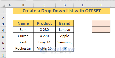
STEP 1: Creating a Drop-Down list in F3
- Go to Data Validation as described in method 1. In Source, create a cell reference: the table headers (B3:D3).
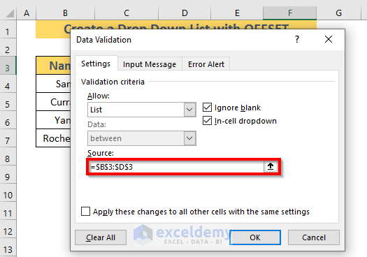
- Excel will create a drop-down list in F3.
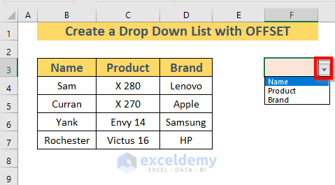
STEP 2: Creating a Dynamic Drop-Down list in F4
- Go to Data Validation as described in method 1. In Source, enter the following formula
=OFFSET($B$3,1,MATCH($F$3,$B$3:$D$3,0)-1,COUNTA(OFFSET($B$3,1,MATCH($F$3,$B$3:$D$3,0)-1,10,1)),1)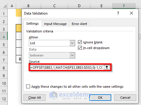
Formula Breakdown
➥ MATCH($F$3,$B$3:$D$3,0) ➜ Returns the relative position of the F3 in B3:D3
Output: {1}.
➥ OFFSET($B$3,1,MATCH($F$3,$B$3:$D$3,0)-1,10,1) ➜ Returns a range based on the row and column of a given reference. The height is 10. The output will be an array of 10 cell values starting from the reference.
Output: {“Sam”;”Curran”;”Yank”;”Rochester”;0;0;0;0;0;0}
➥ COUNTA(OFFSET($B$3,1,MATCH($F$3,$B$3:$D$3,0)-1,10,1)) ➜ Returns the number of cells that are not empty in the selected range.
➥ COUNTA{“Sam”;”Curran”;”Yank”;”Rochester”;0;0;0;0;0;0}
Output: {4}
➥ OFFSET($B$3,1,MATCH($F$3,$B$3:$D$3,0)-1,COUNTA(OFFSET($B$3,1,MATCH ($F$3,$B $3:$D$3,0)-1,10,1)),1) ➔ Returns a range based on the row and column of a given reference
➥ OFFSET($B$3,1,1-1,COUNTA{“Sam”;”Curran”;”Yank”;”Rochester”;0;0;0;0;0;0}),1)
➥ OFFSET($B$3,1,0,4,1)
Output: {“Sam”;”Curran”;”Yank”;”Rochester”}
Explanation: The reference is B3. Since the row is 1 and the column is 0 with a height of 4 cells, the function returns the values in B4:B7.
- Click OK.
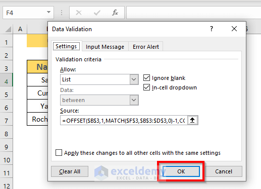
Excel will create a dynamic drop-down list in F4. The options will change depending on the selection in F3. If you select Name in the F3 drop-down list, the drop-down list in F4 will show the names available in the Name column.
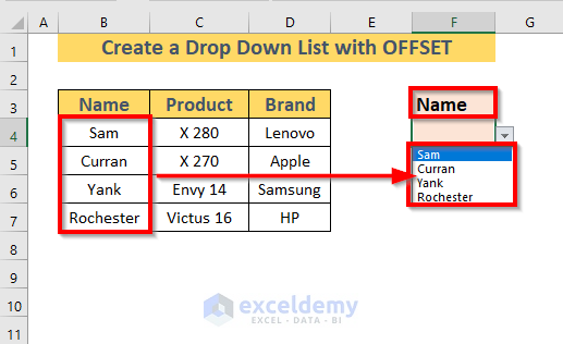
If you select Product in the F3 drop-down list, the drop-down list in F4 will show the products available in the Product column.
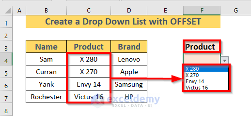
If you add or update the Name, Product, or Brand, Excel will update the drop-down list in F4. A new name Rock was added in the Name column. Excel added the name in the drop-down list.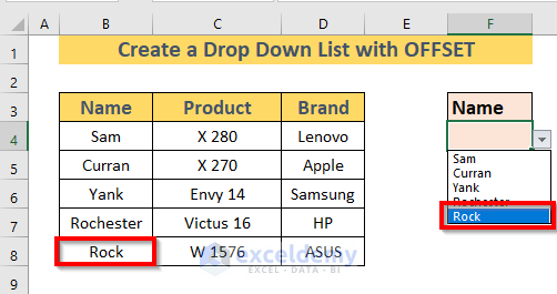
Read More: How to Create a Dynamic Top 10 List in Excel
Practice Workbook
Practice here.
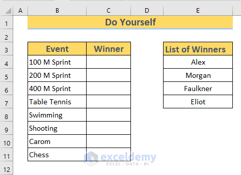
Download Practice Workbook
Related Articles
- How to Create Dynamic List From Table in Excel
- How to Create Dynamic List in Excel Based on Criteria
- How to Make Dynamic Drop Down List from Another Sheet in Excel
<< Go Back to Dynamic List Excel | Excel Drop-Down List | Data Validation in Excel | Learn Excel
Get FREE Advanced Excel Exercises with Solutions!


It doesn’t work in google sheets though. Any ideas on how to fix that?
Hi LILIA,
 \
\
I hope you are doing well.
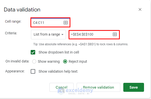
Please use the conditions as per the image and see if it works.
The range $E$4:$E$100 will allow you to have a list of 97 items. So, this can be used as a dynamic drop-down
Thank you.