How to Create an Employee Leave Record Format in Excel

Step 1 – Set Leave Types and Months

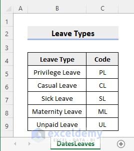
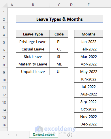
Make a list of the leave types that you allow for your employees. Assign a short code to each type for convenience. The following picture will give you an example.

Create a list of months. You’ll record the leave taken by each employee for each of these months.
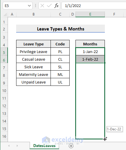
Start with the first month of 2022. Enter the dates 1-Jan-2022 and 1-Feb-2022 in cells E5 and E6, respectively.
Select cells E5:E6 and drag the Fill Handle icon. Excel will recognize that you’re creating a series with a one-month increment, so the month of the date will increase automatically.
Drag the icon until it reaches the desired month. For illustration purposes, let’s drag until 1-Dec-22.

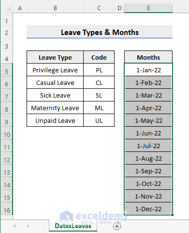
Keep the dates selected.
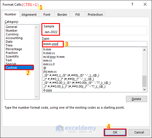
Press CTRL+1 to open the Format Cells dialog box.
Set the Custom Number Format to mmm-yyyy for the dates.
Press OK.

You will get the following result.

Step 2 – Set Months Drop-Down with ComboBox

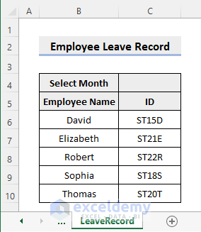
Create a new worksheet named LeaveRecord.
Assume you want to enter employee names in column B and their IDs in column C.

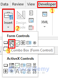
Go to the Developer tab and select Insert and click on Combo Box (Form Control).

Drag the mouse around cell C4 to resize the Combo Box as needed. You can choose another location if necessary.

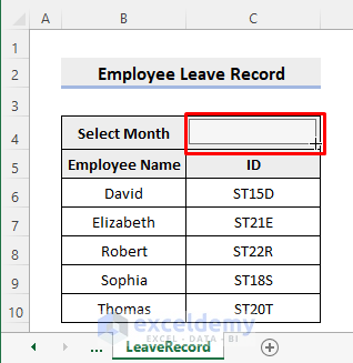
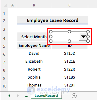
The Combo Box is inserted as follows. Put the cursor on the small circles and drag your mouse to resize the Combo Box if needed.

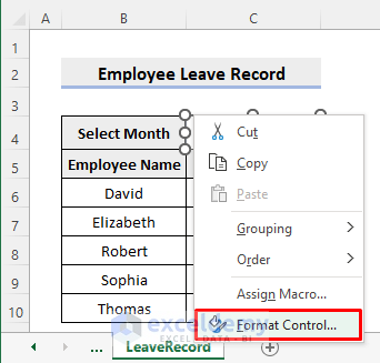
Right-click on the Combo Box and select Format Control.

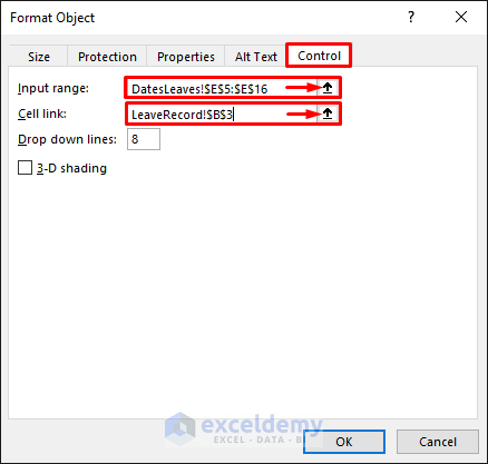
In the Format Object dialog box, go to the Control tab.
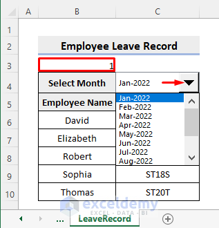
Click the upward arrow in the Input range field and select all the months you generated earlier (from the DatesLeaves list).
Use the upward arrow in the Cell link field to select cell B3 in the current worksheet (LeaveRecord).

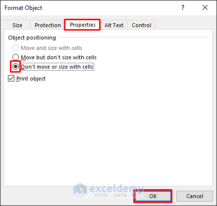
Go to the Properties tab and mark the radio button for Don’t move or size with cells.
Press OK.

You can select any month from the list using the dropdown, and cell B3 will show the order of your selection.

Step 3 – Generate Dates and Days for Selected Month

Enter the following formula in cell C3:

=INDEX(DatesLeaves!E5:E16,LeaveRecord!B3)

- The INDEX function retrieves the date from the list of months based on the order of selection in cell B3.

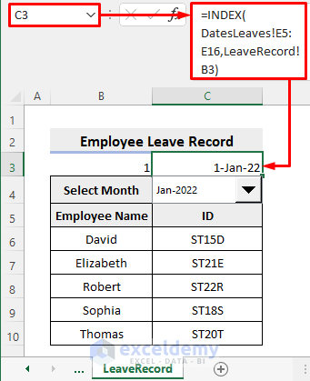
Format cell C3 as d-mmm.
In cell D4, enter the following formula:

=C3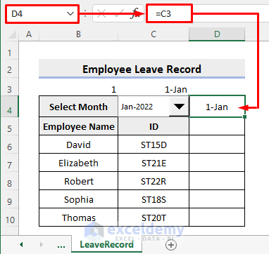

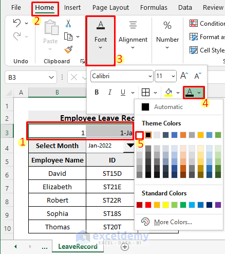
Select cells B3:C3 and change the font color to white.

In cell D5, enter the TEXT function to convert the value to text in the specific number format:

=TEXT(D4,"DDD")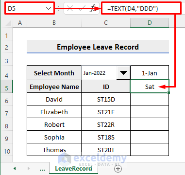

Enter the following formula in cell E4:

=IF(D4="","",IF(EOMONTH($C$3,0)>=D4+1,D4+1,""))

- The EOMONTH function returns the serial number of the last day of the month before or after the specified number of months.

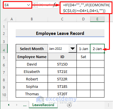
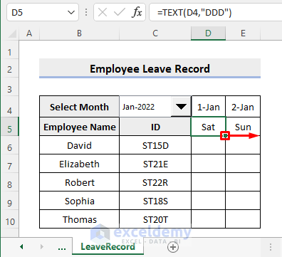
Copy the formula from cell D5 to cell E5 by dragging the fill handle icon.

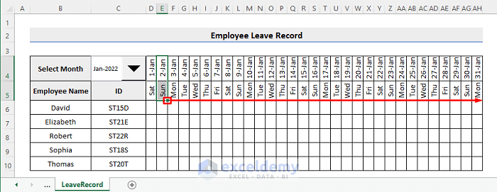
Change the text alignment of cells D4:D5 to vertical (you can do this from the Alignment tab in the Format Cells (CTRL+1) dialog box)).

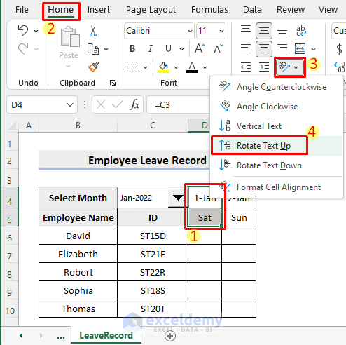
Apply the same alignment to cells E4:E5.
Drag the fill handle icon up to column AH to copy the formulas.

Step 4 – Create Drop-Down to Record Leave

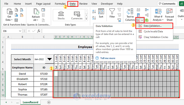
Select the range D6:AH10.
Go to the Data tab and choose Data Validation (ALT+A+V+V).

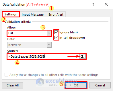
Select List as the validation criteria.
Click the upward arrow in the Source field and select the sort codes for the leave types.
Click OK.

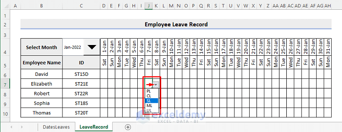
You can choose the leave type using the dropdowns in any of those cells.

Step 5 – Enter Formula to Count Leave

Copy the table for Leave Types and paste it as Transpose onto cell AI4.
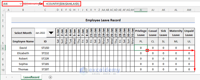
Enter the following formula in cell AI6:

=COUNTIF($D6:$AH6,AI$5)

Drag the fill handle icon from cell AI6 to cell AM6 and then to cell AM10. The COUNTIF function counts the cells based on the specified criteria.

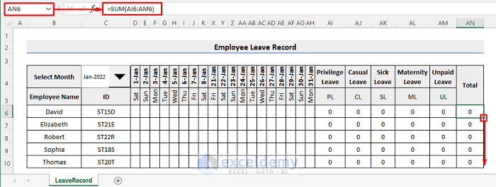
Enter the following formula in cell AN6:

=SUM(AI6:AM6)

Copy the formula down to the cells below.

Step 6 – Format Cells to Hide Zeros

Select the range AI6:AN10.
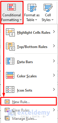
Go to the Home tab, choose Conditional Formatting and select New Rule.

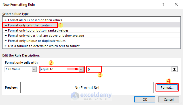
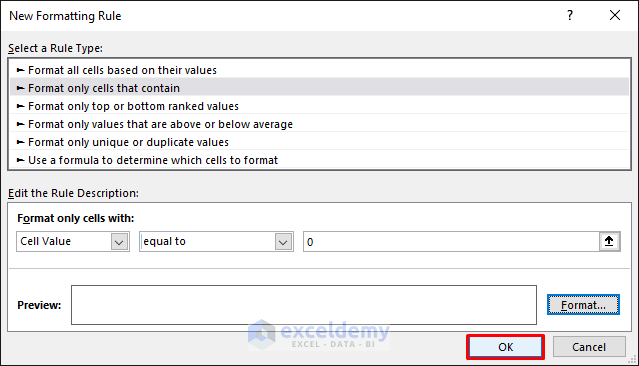
Select the Format only cells that contain rule.
Choose Cell Value, select equal to and enter 0.
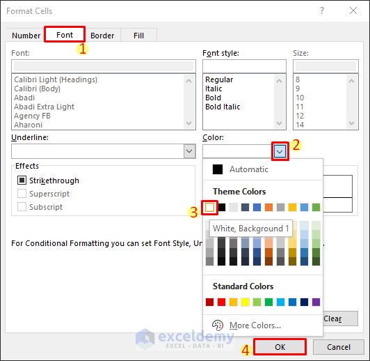
Click on Format and change the font color to white.

Click OK.

Click OK again.

Start recording the leave taken by your employees to see the desired result.

Things to Remember

Be careful while entering the formulas with mixed references to avoid erroneous results.
You can include more rows to record data for additional employees.

Download Sample Workbook

You can download the practice workbook from here:

Employee Leave Record.xlsx

<< Go Back to Excel Employee Leave Tracker | Excel HR Templates | Excel Templates

Get FREE Advanced Excel Exercises with Solutions!

Private Sub Worksheet_Change(ByVal Target As Range) ' Check if the changed cell is D3 If Not Intersect(Target, Me.Range("D3")) Is Nothing Then ' Copy the entire sheet Me.Copy After:=Sheets(Sheets.Count) ' Clear contents of range D6:AH1006 Me.Range("D6:AH1006").ClearContents End If End Sub

16 Comments

V Shanthi Nov 15, 2022 at 11:44 AM

hi good afternoon. the excel leave tracker is very useful but how to add in another column to show the employee’s leave balance and entitlement.
Thanks
- Reply
  Shahriar Nov 16, 2022 at 3:18 PM
  
  Hello V SHANTHI,
  First of all, thanks for your appreciation. Now, let’s get back to your query. Here, you wanted to add a new column for showing the leave balance of employees. If you want to do this on a monthly basis, follow the steps below.
  • At first, create a new column with the heading Leave Balance under Column AO.
  
  • Then, go to cell AO6 and enter the following formula.
  =4-AN6
  Here, we assumed 4 leaves can be taken in a month. It could be changed according to your need.
  • After that, press the ENTER button.
  
  • Now, bring your cursor to the right-bottom corner of cell AO6 and it’ll look like a plus (+) sign. It’s the Fill Handle tool.
  • Afterward, double-click on it.
  
  You can see the results in the following cells also.
  
  On the other hand, if you find out the employee leave balance or remaining leaves on a yearly basis, you can follow the article How to Track Employee Vacation Time in Excel on our website.
  So, that’s all from me on this topic. Please visit our website, ExcelDemy, to explore more. Happy Excelling.
Narendra Jan 18, 2023 at 4:10 PM

Hi, Shamim raza
based on the above formula’s I create a template it is good, but i have one doubt when we change the months, that leave record doesn’t change, when we add next month leaves its overlap, please give a suggetion for that
- Reply
  Rafiul Haq Jan 25, 2023 at 11:31 AM
  
  You can duplicate the months below the first month for multiple months’ data. Moreover, if you need to remove the values, you can just click the cell range and hit the Delete button. I have added the leave record format for four months in the following file. This can be found on the LeaveReord sheet.
  Leave Record for User
  - Reply
    Ayesha Feb 3, 2023 at 5:05 PM
    
    So we will have to create separately for each month?
    - Lutfor Rahman Shimanto Feb 6, 2023 at 12:00 PM
      
      Hello AYESHA
      Thanks for your query. I have analyzed the workbook Rafiul Haq shared. A prominent approach to avoid data overlapping is to create the employee record separately for each month. So don’t hesitate to make the Employee Leave description for each month.
      Regards
      Lutfor Rahman Shimanto
maheswari Jan 27, 2023 at 2:18 PM

need 2023 leave record excel
- Reply
  Arin Jan 30, 2023 at 1:04 PM
  
  Hi MAHESWARI,
  Thank you for your comment.
  To create a leave record for 2023 in Excel you can follow the steps given in the article with some little changes.
  • First of all, insert 1-Jan-2023 and 1-Feb-2023 in Cell E5 and E6.
  • Then, drag the icon until it reaches the desired month. Here, we will drag until 1-Dec-23 for illustration.
  
  • Next, you will get the following result.
  
  • After that, follow the same steps shown in the article and you will be able to create a leave record for 2023.
  
  We hope this will solve your problem. Please let us know if you face any further problems.
  
  Regards,
  Arin Islam,
  ExcelDemy
Aamir Feb 27, 2023 at 2:04 PM

how to record half day casual leave ?
- Reply
  Afia Kona Mar 1, 2023 at 1:10 PM
  
  Dear AAMIR
  Thank you for your comment.
  If you want to make a recorder for only half-day casual leave, you can use the same template in this article. In this case, each “1” will be a half-day leave. And the total will imply a total half day’s leave. Change the header for your needs.
  
  Also, for better reach, you can review the following article to record a half-day casual leave.
  https://www.exceldemy.com/calculate-half-day-leave-in-excel/
  
  Best,
  Afia Aziz Kona
Nn Aug 7, 2023 at 10:36 AM

Hi,
I have followed the instructions and created the Leave record sheet but when i change the months, for eg: Jan leaves are entered and when i change the month to Feb from the created drop down months the listed Jan leaves appear on the feb sheet and all other months sheet as well. Please help me rectify this issue.
- Reply
  Sourav Kundu Aug 8, 2023 at 3:16 PM
  Hi NN,
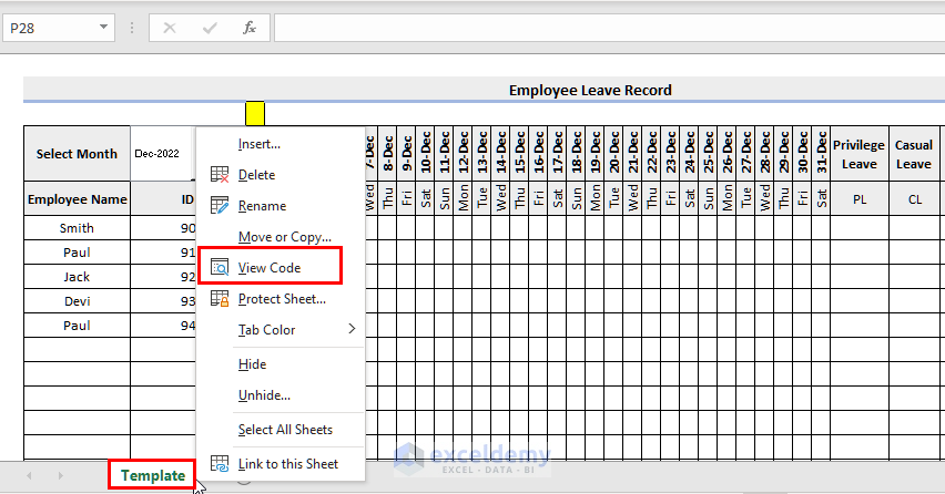
  Thank you for sharing your problem with us. We have got a solution to your requirement. With this solution, whenever you need a blank record, you just have to change the value of the yellow-colored cell. You have to use a VBA code in the worksheet for the purpose.
  First, Right-click on your worksheet named Template.
  Then, click on View Code.
  
  Then. copy the following VBA code and paste it into the opening window:
```
Private Sub Worksheet_Change(ByVal Target As Range)
    ' Check if the changed cell is D3
    If Not Intersect(Target, Me.Range("D3")) Is Nothing Then
      ' Copy the entire sheet
      Me.Copy After:=Sheets(Sheets.Count)
      ' Clear contents of range D6:AH1006
      Me.Range("D6:AH1006").ClearContents
    End If
End Sub
```
  Now, go back to your workbook and insert some Employee Leaves.
  Now, write something say N, and press Enter.
  
  The code will create a new worksheet containing the Employee Leaves records.
  
  Now, go back to the previous worksheet.
  The original worksheet is blank and is ready to take instructions from scratch.
  
  Note: You can change the Yellow color cell reference from the VBA code.
  You can download the updated template with the VBA code from below:
  Answer.xlsm
  We hope that we have provided a reasonable solution to your problem. If you have more queries you can always mention them in the comment section.
  
  Regards,
  Sourav Kundu
  Exceldemy.
Soumendra Sep 6, 2023 at 8:45 PM

This is excellent way of track your leave records., many appreciations,
- Reply
  Shamima Sultana Sep 7, 2023 at 9:51 AM
  
  Dear Soumendra
  
  You are most welcome.
  
  Regards
  ExcelDemy
LinebetApp Oct 22, 2024 at 7:36 PM

Great post! The step-by-step instructions made it really easy to create a leave record in Excel. I especially appreciated the template you provided. This will definitely help keep track of employee leaves more efficiently. Thank you!
- Reply
  Shamima Sultana Oct 22, 2024 at 8:06 PM
  
  Hello,
  
  You are so welcome. Thanks for your feedback and appreciation. Glad to hear that the step by step instructions made it easy to create a leave record. Keep learning Excel with ExcelDemy!
  
  Regards
  ExcelDemy