How to Use the ABS Function in Excel – 12 Examples

This is an overview:

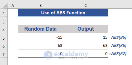
Introduction to ABS Function

Function Objective:

The ABS function is used to get the absolute value of a number. You will get only a positive number.

Syntax:

=ABS(number)

Argument:

Returns:

A number with a positive sign.

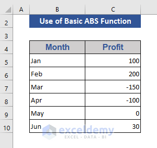
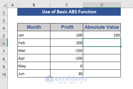
The sample dataset showcases of a store’s profit in the 1st six months of 2021.

To get the absolute results in this dataset:

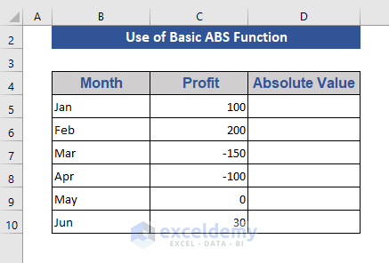
Step 1:

• Add a column: Absolute Value.

Step 2:

• Enter the ABS function in D5. Use C5 as the argument. The formula is:

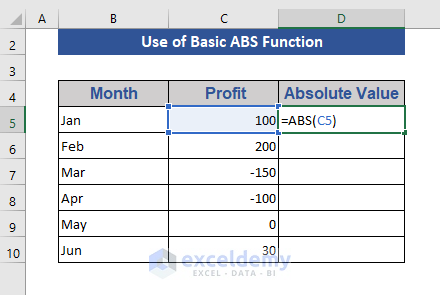
Step 3:

• Press Enter.

Step 4:

• Drag down the Fill Handle to see the result in the rest of the cells.

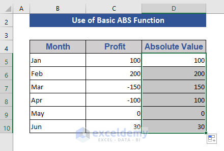
All objects are positive in the Result section. The ABS function affects the negative numbers only. It has no impact on positive numbers and zeros. It converts negative numbers into positive ones.

Example 1 – Find the Absolute Variance Using the ABS Function

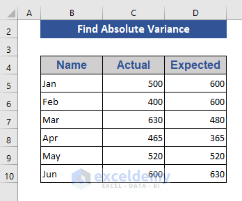
Step 1:

• Enter the actual and expected revenue:

Step 2:

To see the difference between the actual and expected revenue in the Error column:

• Enter the formula in the Error column. Drag down the Fill Handle to see the result in the rest of the cells.

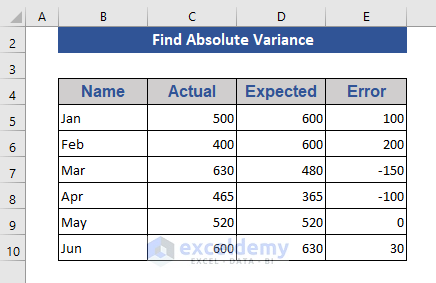
This difference is the variance. There both positive and negative values.

Use the ABS function to see the absolute variance:

Step 3:

• Enter the ABS function in the Error column:

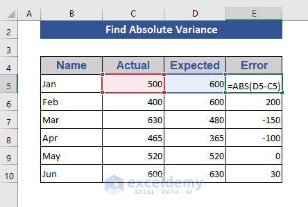
Step 4:

• Drag down the Fill Handle to see the result in the rest of the cells.

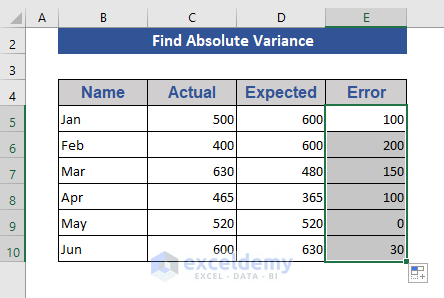
The absolute variance is displayed.

Example 2 – Get the Absolute Variance with a Condition using the ABS Function

Find the absolute variance with conditions using the SUMPRODUCT function with the ABS function.

Step 1:

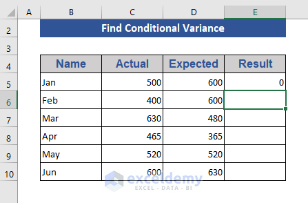
• Add a column (Result) to see the conditional variance.

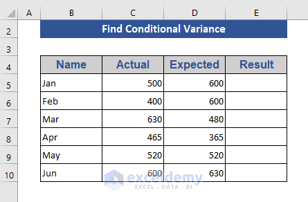
Step 2:

• Enter the formula in E5:

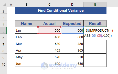
A condition is set: 1 for a variance value greater than 100. Otherwise, 0.

Step 3:

• Press Enter.

Step 4:

• Drag down the Fill Handle to see the result in the rest of the cells.

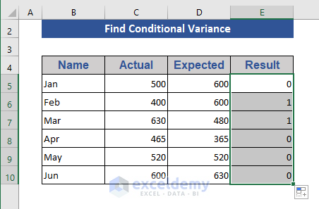
This is the output.

Example 3 – Find the Square Root of a Negative Number using the ABS Function

Use the SQRT function and the ABS function.

Step 1:

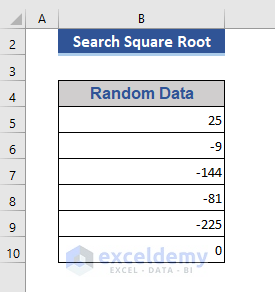
• This is the sample dataset.

Step 2:

• Enter the SQRT formula in C5:

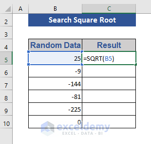
Step 3:

• Press Enter and drag down the Fill Handle.

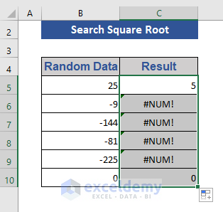
The SQRT function displays errors for the negative numbers.

Step 4:

• Use the ABS function:

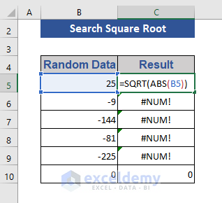
Step 5:

• Press Enter and drag down the Fill Handle.

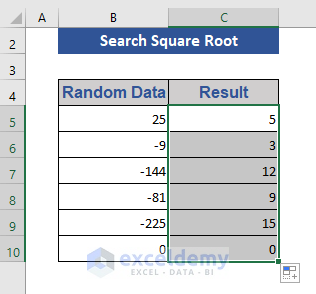
The square root is displayed, including the negative values.

Example 4 – Using the ABS Function to Find the Tolerance in Excel

Use the ABS function and the IF function.

Step 1:

• Create a column to display the result.

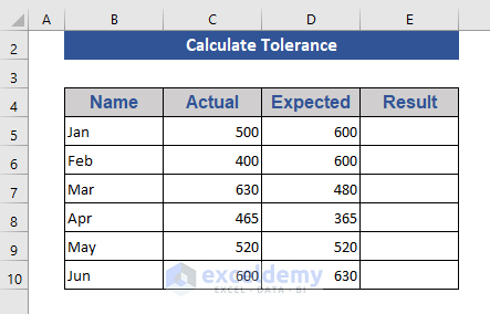
Step 2:

• Enter the formula in E5:

• Tolerance was set to 100.

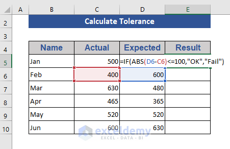
Step 3:

• Press Enter.

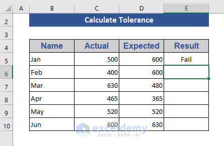
Step 4:

• Drag down the Fill Handle to see the result in the rest of the cells.

Cells below the tolerance level show OK. Otherwise, Fail.

Example 5 – SUM Numbers Ignoring Their Signs with the ABS Function

Step 1:

• Find the sum of these random numbers:

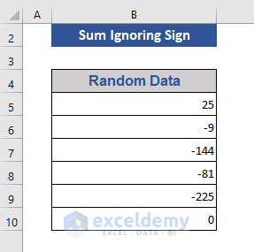
Step 2:

• Enter the formula in B12:

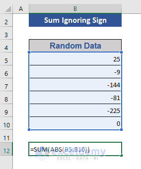
Step 3:

• Press Ctrl+Shift+Enter, as this is an array formula.

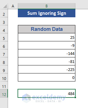
The total is displayed without signs.

Read More: How to Sum Absolute Value in Excel

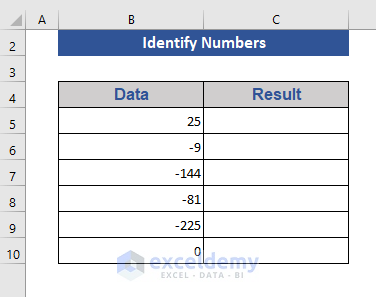
Example 6 – Return an Absolute Value of Negative Numbers and Identify the Non-negative numbers

Step 1:

• Insert a column to see the result.

Step 2:

• Enter the formula in C5:

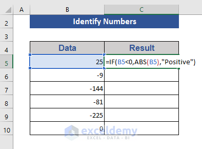
Step 3:

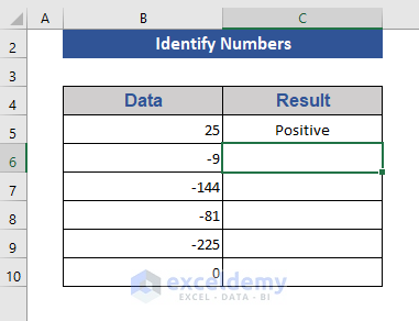
• Press Enter.

Step 4:

• Drag down the Fill Handle to see the result in the rest of the cells.

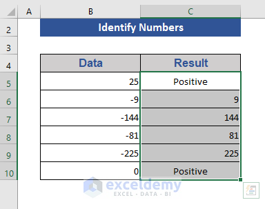
You get the absolute value for negative numbers. For non-negative numbers Positive is displayed.

Read More: Changing Negative Numbers to Positive in Excel

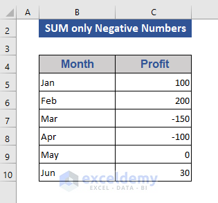
Example 7 – SUM the Negative Numbers Only with the ABS Function in Excel

Use the SUM and the IF functions here.

Step 1:

• To sum the negative numbers in the data below:

Step 2:

• Enter the formula in C12:

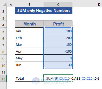
Step 3:

• Press Enter.

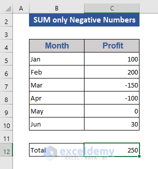
This is the output.

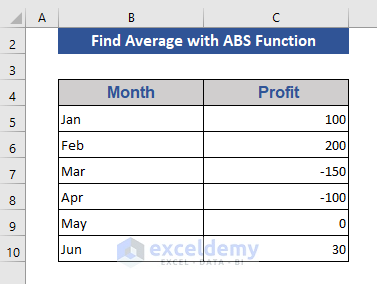
Example 8 – Get the Average of Absolute Values using the Excel ABS Function

Use the Average function.

Step 1:

• To find the average profit in the dataset below:

Step 2:

• Enter the formula in C12:

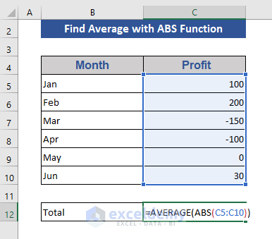
Step 3:

• Press Ctrl+Shift+Enter.

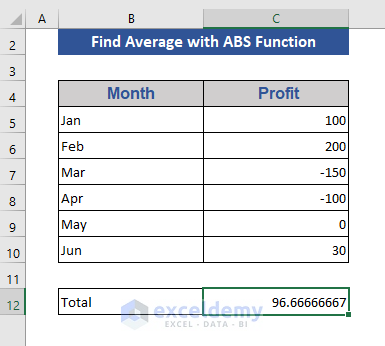
This is the output.

Example 9 – Find the Maximum/Minimum Absolute Value in Excel

The dataset showcases temperatures in different states. To find the maximum absolute temperature, use the MAX and the ABS functions.

To find the minimum absolute value, use the MIN and the ABS functions.

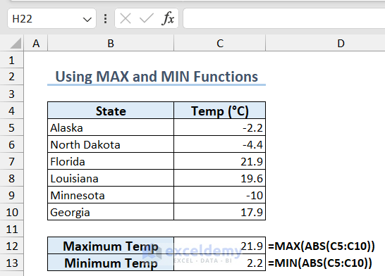
Example 10 – Calculate the Closest Even Number of Given Numbers

To calculate the closest even number of the given numbers, use the IF, EVEN and ABS functions.

Use the following formula:

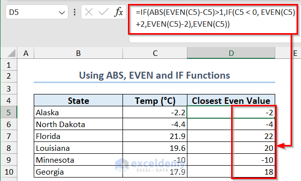
Example 11 – Identify the Closest Value from a List of Values in Excel

To identify the closest value to  a specific value from a given list, use the INDEX, MATCH, MIN and ABS functions.

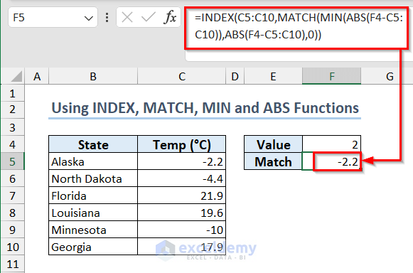
Example 12 – Calculate the Absolute Value Using the ABS Function in VBA

Use the ABS function in VBA Macros.

Step 1:

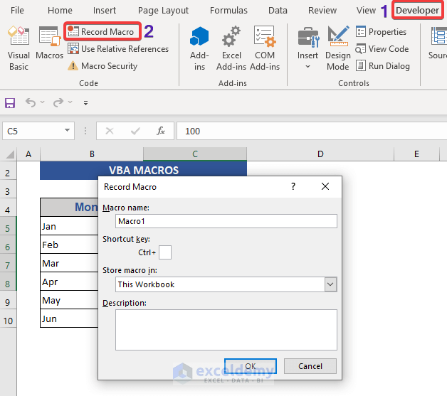
• Go to the Developer tab.
• Select Record Macros.

Step 2:

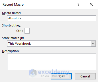
• Set Absolute as the Macro name.
• Click OK.

Step 3:

• Enter the VBA code.

Sub Absolute()
Rng = Selection
XML = ""
For Each i In Rng:
n = Abs(i)
X = X + Str(n) + vbNewLine + vbNewLine
Next i
MsgBox X
End Sub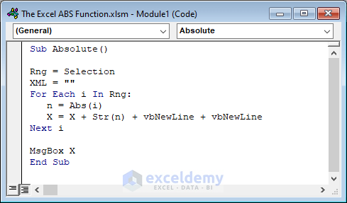

Step 4:

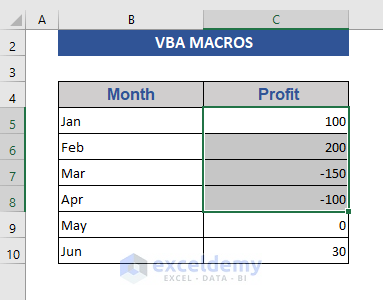
• Select the cells.

Step 5:

• Press F5.

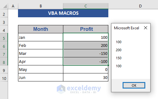
The selected range is C5:C8.

Things to Remember

• In an array function, press Ctrl+Shift+Enter instead of Enter.
• Only numeric values can be used with this function.

Frequently Asked Questions

1. Can the ABS function be nested within other functions?

Yes, you can use it as part of a larger formula.

2. How does the ABS function handle zero?

The ABS function treats zero as a non-negative number, so ABS(0) will return 0.

Download Practice Workbook

Download the practice workbook.

ABS Function in Excel: Knowledge Hub

• How to Get Absolute Value in Excel
• How to Make All Numbers Positive in Excel
• How to Calculate Absolute Difference between Two Numbers in Excel
• Opposite of ABS Function in Excel
• Calculate Absolute Percentage Error with Excel Function

<< Go Back to Excel Functions | Learn Excel