Method 1 – Modify Cell Format
Steps
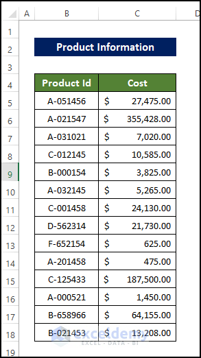
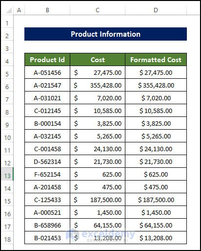
- We have the Product Information in the range of cells B4:C14.
- And the costs in column C are right aligned.
- Now if we try to change the alignment of the cells, such as center alignment, there is no alignment change at all. The alignment seemed to be static at this point.
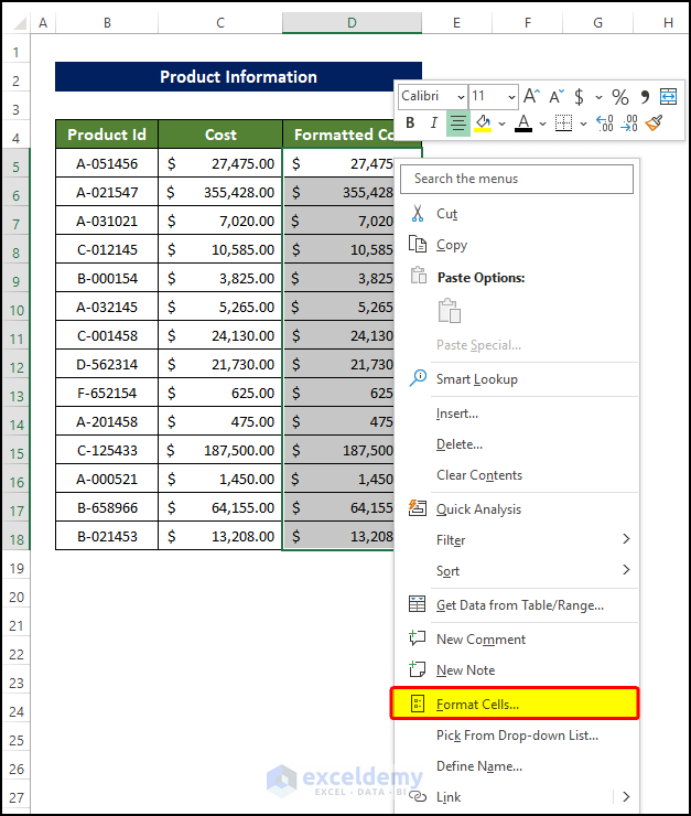
- Copy the cells in the range of cells D5:D18, right-click on the mouse.
- From the context menu, click on Format Cells.
- A new window named Format Cells will open.
- Go to the Number tab.
- Click on the Custom option.
- You can see the Custom formatting text in the right-side menu, which defines your cell values format.
- In the type of field, you will notice a small asterisk in between the text (marked with an arrow sign in the image below).
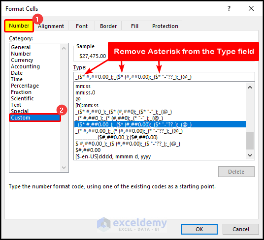
- Remove those asterisks one by one.
- Click OK.
- The final formatting will look like the one below.
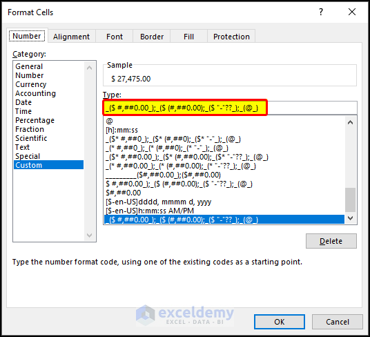
- After clicking OK, you will notice that the alignment is now in correction alignment.
Method 2 – Change Custom Number Formatting
Steps
- We got the unit price in the product information dataset.
- The Unit Price values are slightly right aligned, and we actually want to align it as the center.
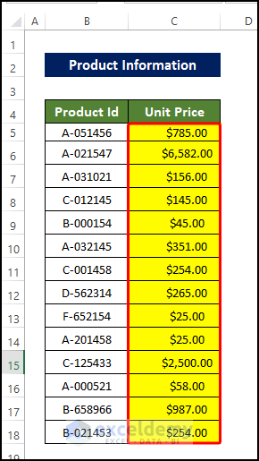
- First, copy the values in the Unit Price in the D5:D18 range.
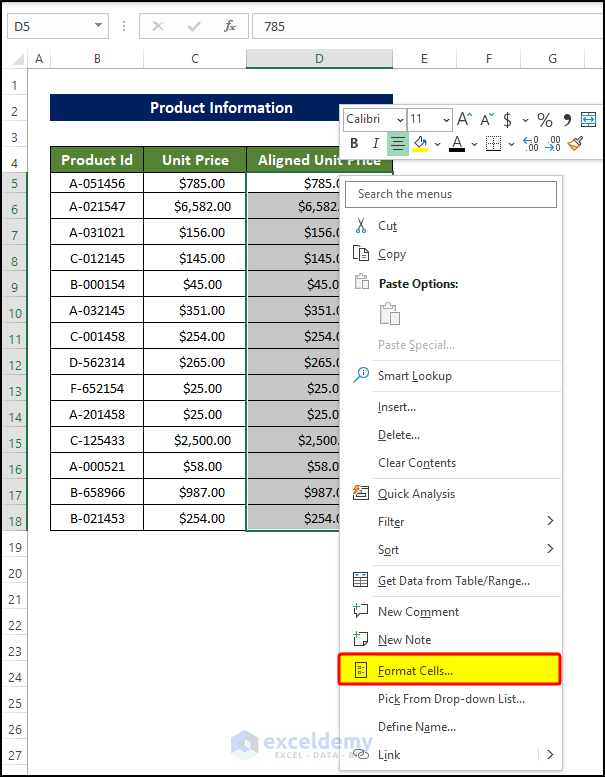
- Right-click on the Unit Price values.
- From the context menu, click Format Cells.
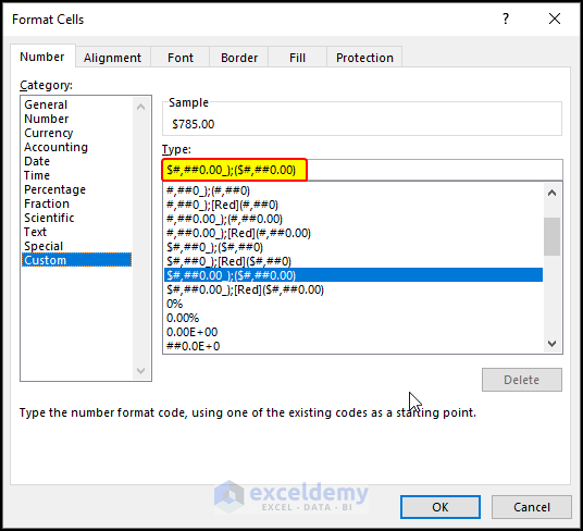
- In the Format Cells new window, click the Number tab, then click Custom.
- In the Type field, notice the spaces before the format texts.
- Click OK after this.
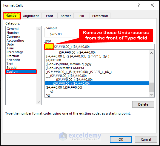
- The final format text will look like the below image.
- Click OK after this.
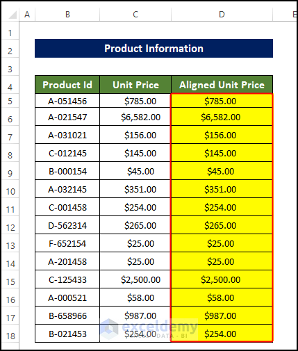
- The Unit Prices column is center-aligned.
Method 3 – Use Text to Columns Command
Steps
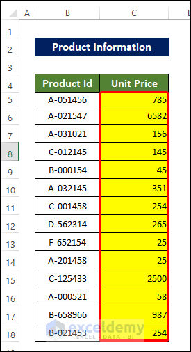
- In the dataset shown below, the cell values are right aligned.
- The main issue here is that they are saved as text vs. number.
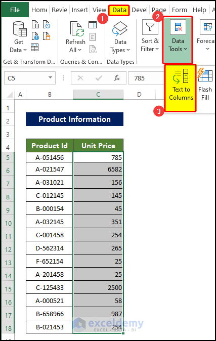
- The ribbon menu, click the Data tab, and then click on Data Tools.
- From the dropdown menu, click the Text to Columns commands.
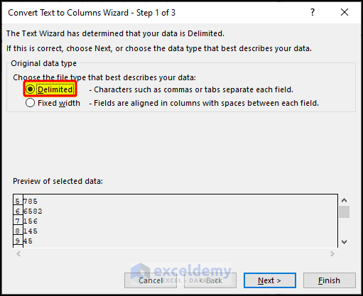
- A new window named the Convert Text to Columns Wizard will open.
- From the Choose the file type that best describes your data, select Delimited.
- Click Next after this.
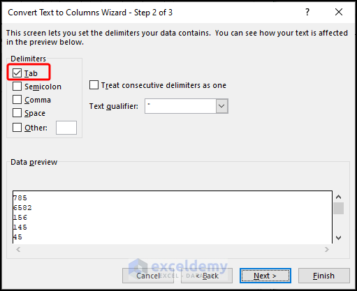
- Check the Tab box if it is not checked.
- Click Next again.
- Select Text and then click Finish.
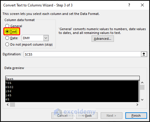
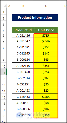
- You can change the alignment of the cells in the worksheets.
- We finally changed the alignment to the center.
Note:
While changing the data format to text, the signs from the original format may be lost. To circumvent this, you need to input the signs inside the cell manually. In this example, the Unit Price. Values contain the 4 signs as part of their formatting. After the data formatting, the $ sign vanished, and we had to manually input the $ sign inside the cells.
Method 4 – Make Sure Cells Are Not Merged
Steps
- Sometimes some cells in the Excel sheets appear to be not in alignment properly.
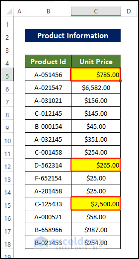
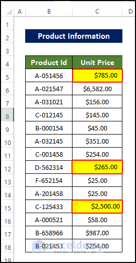
- Notice the below values in the sheet.
- The values of $785, $265, and $2500 now have the proper alignment of the cell. And the rest of the cell values are in central alignment.
- The cells could not be properly aligned.
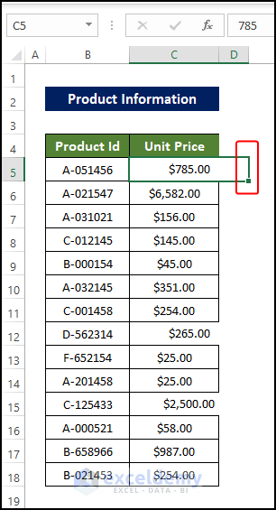
- The $785 and others cell is merged with the neighbor cell.
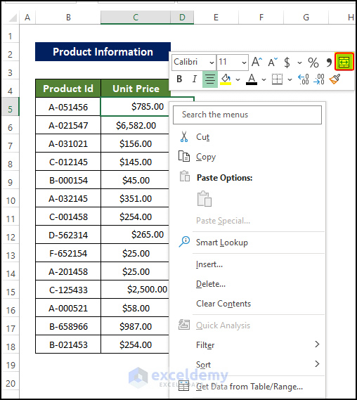
- It can be seen by hovering over the cell as the Fill Handle covers the D5.
- These combined, merged cells are in center alignment. If placed side by side, they appear to be right-aligned compared to other cell values.
- This is the same thing for other cells.
- This, we need to unmerge the cells.
- Select the cells and right-click on the mouse.
- In the context menu, notice the merge/unmerge icon in the corner.
- Click this icon to unmerge the cell in the sheet.
- Do the same for the other cells.
- You can speed up the process by selecting all the cells with these alignment issues and then clicking on the merge/unmerge icon from the context menu.
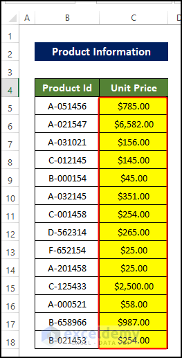
- After clicking the Unmerge icon, you can notice that the cells are now unmerged.
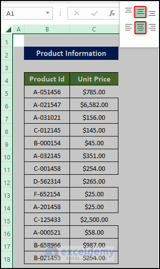
- You can now change the alignment of the cells.
- We can change the alignment to center by clicking on the alignment’s options in the Alignment group in the ribbon.
- All the cells in the Unit Price column have the center alignment.
Method 5 – Use the Copy-Paste Feature to Copy an Alignment
Steps
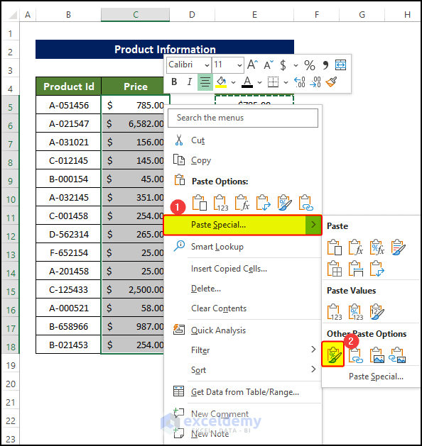
- The cell format of the E5 is now implemented in the range of cells C5:C18.
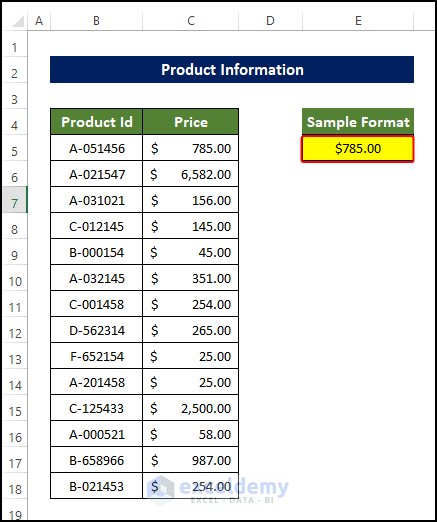
- Copy cell E5.
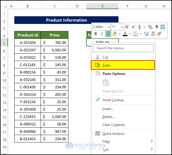
- Select cell C5:C18, and paste the format.
- Right-click on the range of cells C5:C18, and from the context menu, go to Paste Special > Other Paste Option > Paste Format.
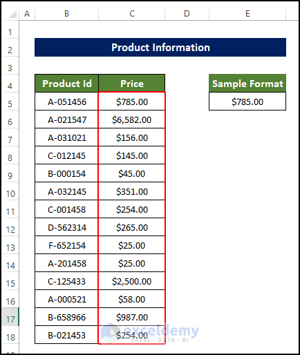
- As the Sample Format cell E5 is in the center-aligned state, the pasted cells are also in the center-aligned state.
Download Practice Workbook
Download this practice workbook below.
Related Articles
- How to Left Align in Excel
- How to Top Align in Excel
- Align Two Sets of Data in Excel
- How to Bottom Align in Excel
<< Go Back to Alignment in Excel | Excel Cell Format | Learn Excel
Get FREE Advanced Excel Exercises with Solutions!
