How to Check If Value Exists in Range in Excel (8 Ways)

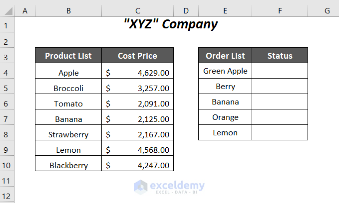
We have the Product List and the Order List of the products of a company, and we want to check if the products of the Order List are available in the Product List.

Method 1 – Using the COUNTIF Function to Check If a Value Exists in a Range

We will get the results as TRUE or FALSE in the Status column.

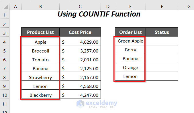
Steps:

• Use the following formula in cell F4

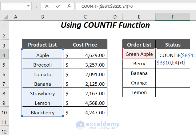
• Press Enter and drag down the Fill Handle tool.

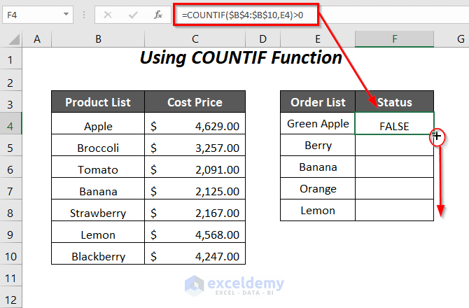
• Here are the results.

Method 2 – Using IF and COUNTIF Functions to Check If a Value Exists in a Range

We’ll use the same dataset. We’ll return custom texts as results.

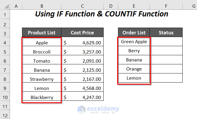
Steps:

Use the following formula in cell F4

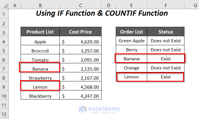
For the result TRUE, we will get Exist and for FALSE we will get Does not Exist.

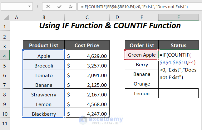
• Press Enter and drag down the Fill Handle tool.

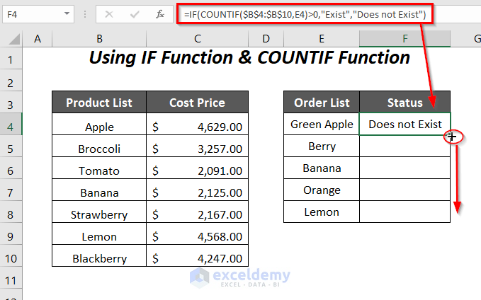
Here are the results.

Method 3 – Checking a Partial Match of Values in a Range

We will check the partial match of the products. We’ve modified the dataset a bit.

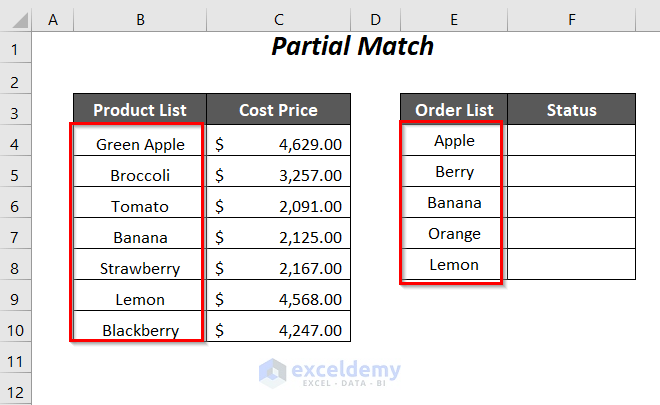
Steps:

• Use the following formula in cell F4

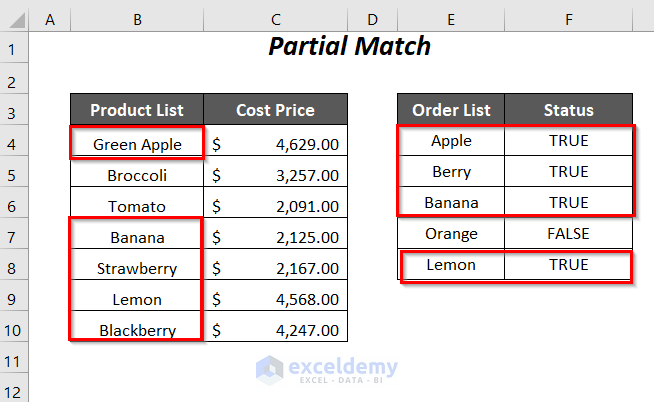
Adding the Asterisk symbol before and after the value of cell E4 will account for zero or more other characters around it.

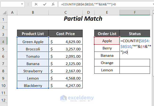
• Press Enter and drag down the Fill Handle tool.

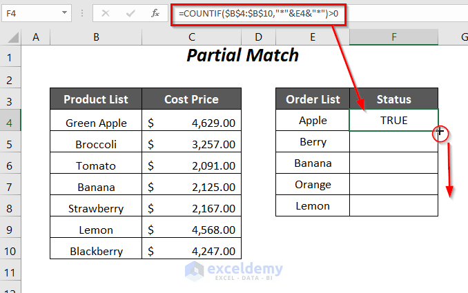
• Here are the results.

Method 4 – Using ISNUMBER and MATCH Functions to Check If a Value Exists in a Range

We’ll use the same dataset.

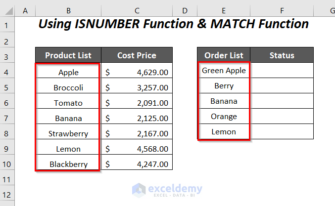
Steps:

• Use the following formula in cell F4

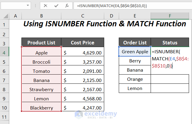
• Press Enter and drag down the Fill Handle tool.

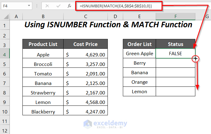
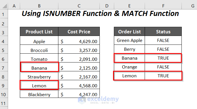
• Here are the results.

Read More: How to Use Excel IF Function with Range of Values

Method 5 – Check If a Value Exists in a Range Using IF, ISNA, and VLOOKUP Functions

We’ll use the same dataset.

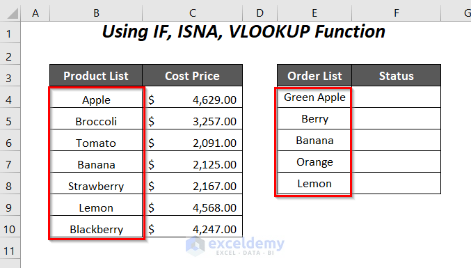
Steps:

• Use the following formula in cell F4

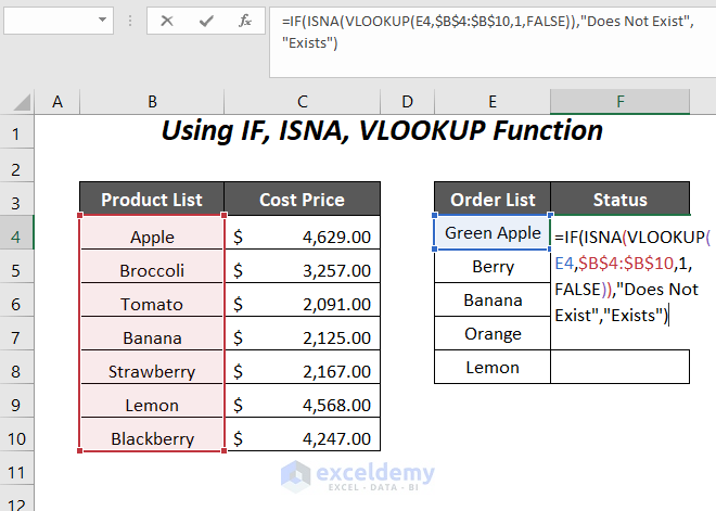
• Press Enter and drag down the Fill Handle tool.

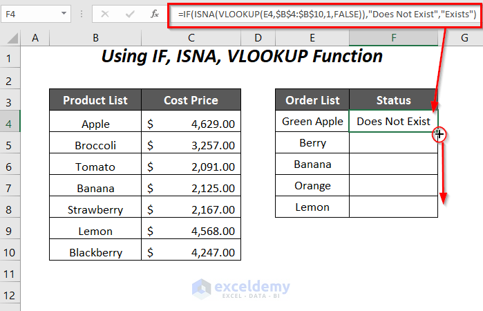
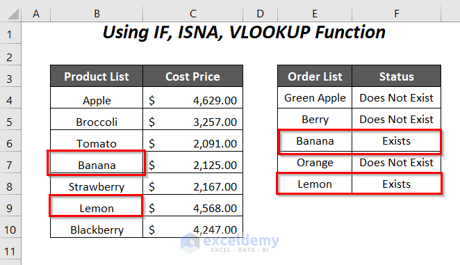
• Here are the results.

Method 6 – Using IF, ISNA, and MATCH Functions to Check If a Value Exists in a Range

We’ll use the same dataset.

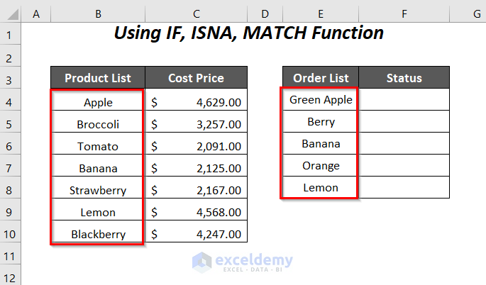
Steps:

• Use the following formula in cell F4

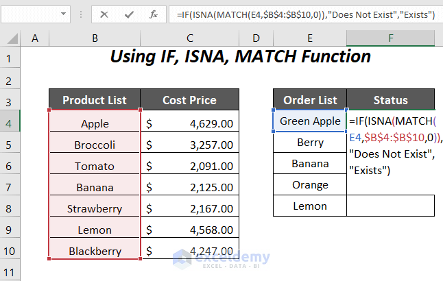
• Press Enter and drag down the Fill Handle tool.

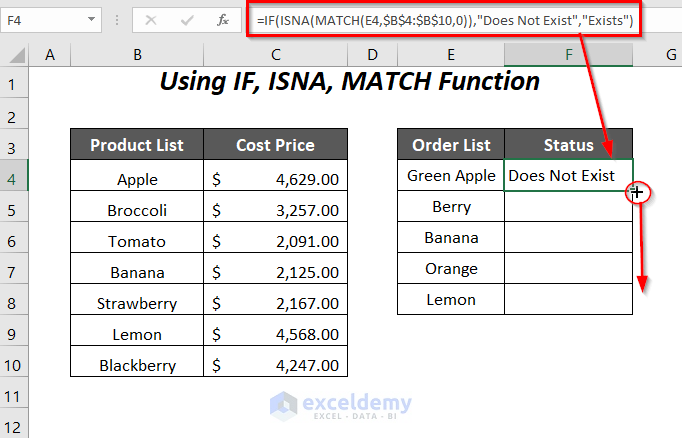
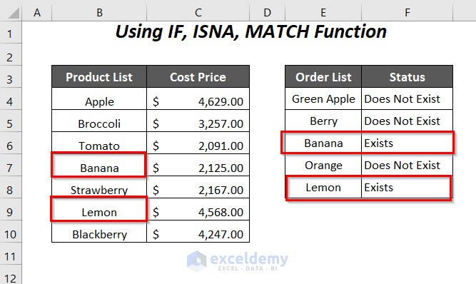
• Here’s the result.

Method 7 – Conditional Formatting to Check If Value Exists in Range

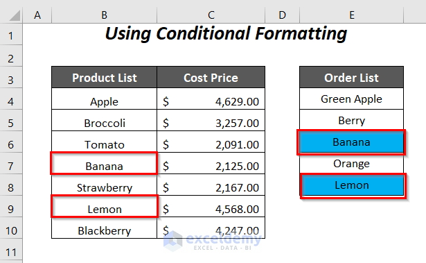
We will highlight the products in the Order List column if they are available in the Product List column.

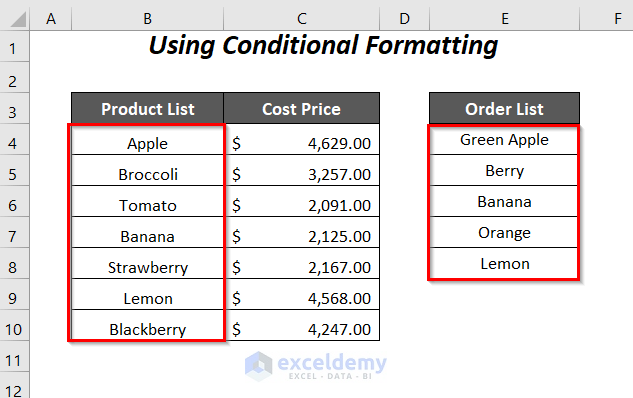
Steps:

• Select the cell range on which you want to apply the Conditional Formatting (We have selected the column Order List).
• Go to the Home tab, choose Conditional Formatting, and select New Rule.

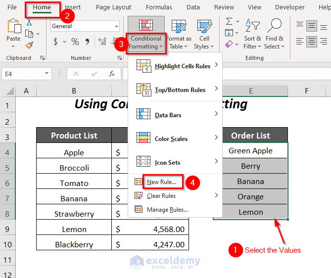
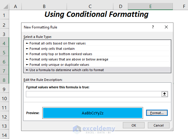
• The New Formatting Rule wizard will appear.
• Select Use a formula to determine which cells to format, and click the Format option.

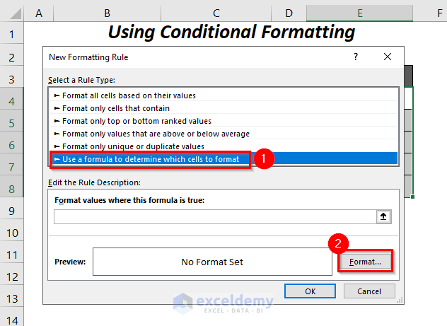
• The Format Cells dialog will open.
• Select the Fill tab.
• Choose any Background Color and click on OK.

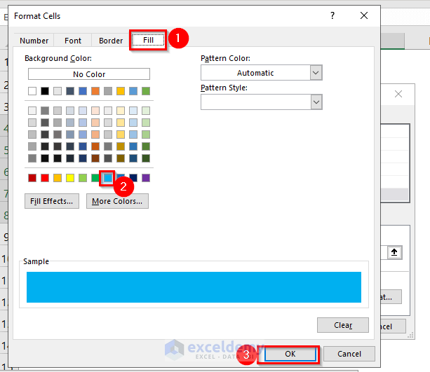
• The Preview will be shown as below.

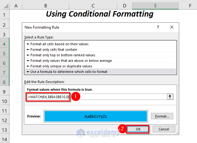
• Use the following formula in the Format values where this formula is true box:

• Press OK.

• This highlights all the cells that fill the formula’s criteria.

Read More: How to Use IF Function with Multiple Conditions in Excel

Method 8 – Using VBA Code to Check If a Value Exists in a Range in Excel

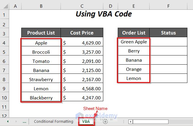
We’ll use the same starting dataset.

Steps:

• Go to the Developer tab and select Visual Basic.

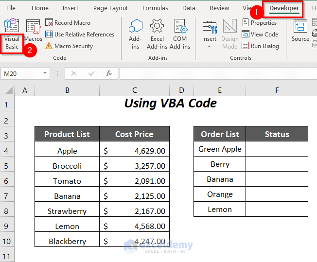
• The Visual Basic Editor will open.
• Go to the Insert tab and select Module.

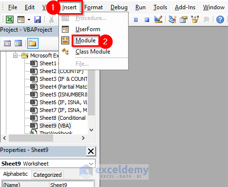
• A Module will be created.

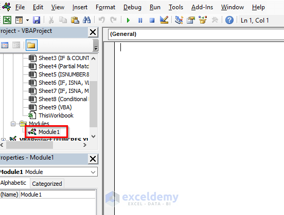
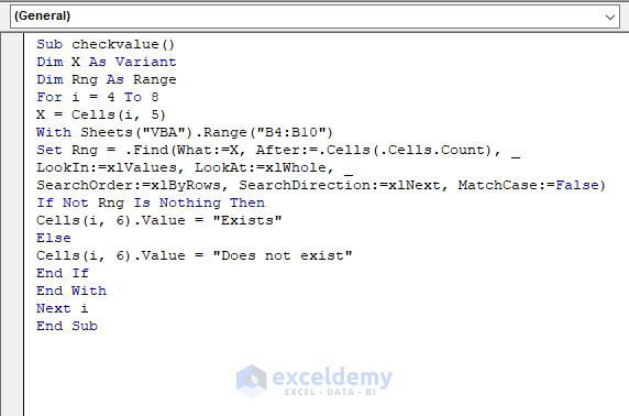
• Insert the following code in the module:

Sub checkvalue()

Dim X As Variant
Dim Rng As Range

For i = 4 To 8
X = Cells(i, 5)
With Sheets("VBA").Range("B4:B10")
Set Rng = .Find(What:=X, After:=.Cells(.Cells.Count), _
LookIn:=xlValues, LookAt:=xlWhole, _
SearchOrder:=xlByRows, SearchDirection:=xlNext, MatchCase:=False)
If Not Rng Is Nothing Then
Cells(i, 6).Value = "Exists"
Else
Cells(i, 6).Value = "Does not exist"
End If
End With
Next i

End Sub

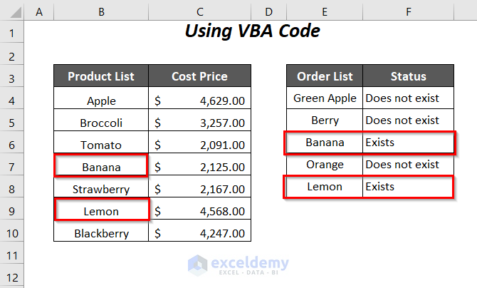
We have declared X as Variant, Rng as Range, and here, VBA is the sheet name.

The FOR loop will execute the operations for each row of the column Order List from Row 4 to Row8, Range(“B4:B10”) is the range of the Product List column. X is assigned to the values of each cell of the Order List column and after finding the matching by using the FIND function we will get Exists in the adjacent cell of the corresponding cell of this column. For not finding the value it will return Does not exist.

• Press F5.

Practice Section

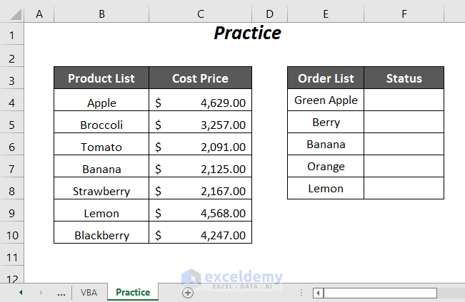
We have provided a Practice section like below in a sheet named Practice.

Download the Practice Workbook

Related Articles

<< Go Back to Excel IF Function | Excel Functions | Learn Excel