Suppose we have the dataset of students’ exam marks below. We want to know whose mark is between 40 and 60. In this article, we will use different formulas and methods to check if the value is between the two numbers.
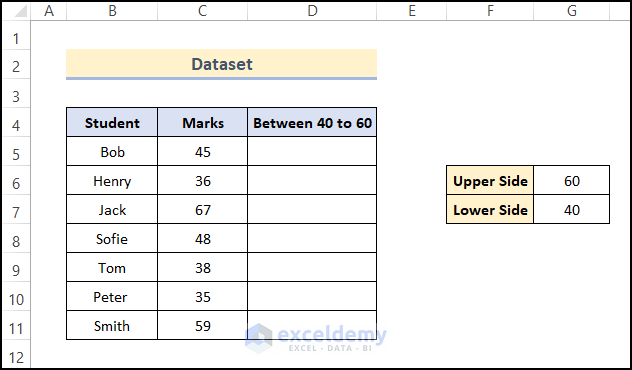
We used Microsoft 365 version, but the methods should work in other versions.
Method 1 – Using the IF Function
Steps:
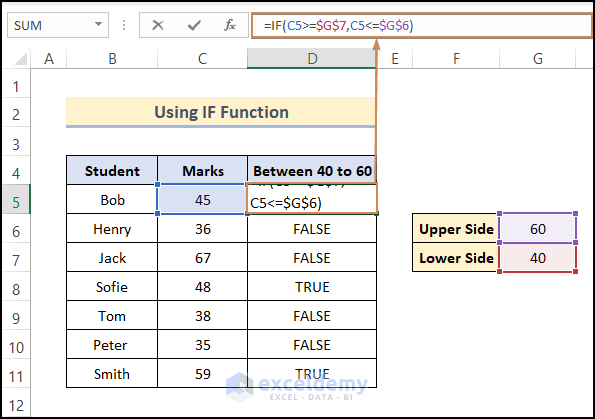
- Select cell D5 and enter the formula below:
=IF(C5>=$G$7,C5<=$G$6)
Here,
C5 = Mark of the student.
G7 = Lower limit.
G6 = Upper limit.
- Press ENTER.
The syntax =IF(C5>=$G$7,C5<=$G$6) checks if the value of C5 lies between the values in cells G6 and G7. If the condition is met, the formula will return TRUE, else FALSE.
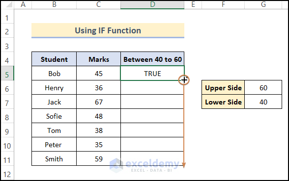
- Drag down the Fill Handle tool to copy the formula to the cells below.
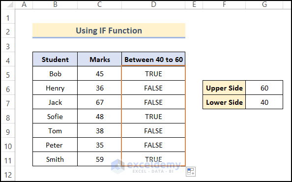
The result looks as below.
Method 2 – Using the AND Function
Steps:
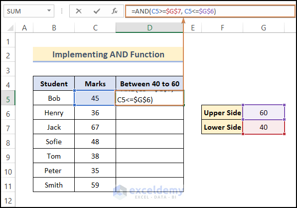
- Select cell D5 and enter the following formula:
=AND(C5>=$G$7, C5<=$G$6)
Here,
C5 = Mark of the student.
G7 = Lower limit.
G6 = Upper limit.
- Press ENTER.
The syntax =AND(C5>=$G$7,C5<=$G$6) checks if the value of cell C5 lies between the values in cells G6 and G7. If the condition is met, the formula will return TRUE, else FALSE.
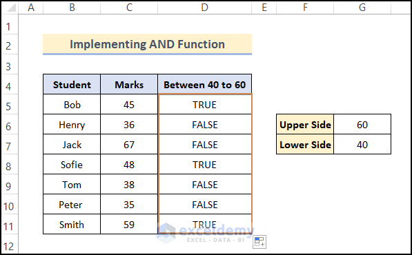
- Drag down the formula to the rest of the cells using the Fill Handle.
The correct results are returned.
Method 3 – Combining the IF and AND Functions
Steps:
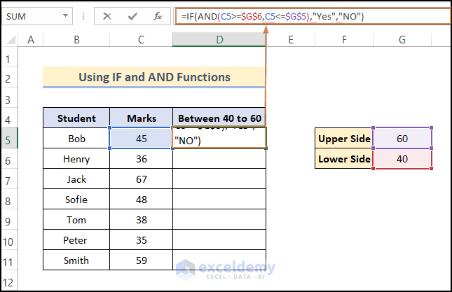
- Enter the following formula in cell D5:
=IF(AND(C5>=$G$6,C5<=$G$5),”Yes”,”NO”)
C5 = Mark of the student.
G7 = Lower limit.
G6 = Upper limit.
- Press ENTER.
Formula Breakdown:
AND(C5>=$G$6,C5<=$G$5)→checks whether the value of C5 lies between the values in cell G5 and G6.
IF(AND(C5>=$G$6,C5<=$G$5),”Yes”,”NO”)→If the condition is met then it will return YES else it will return NO.
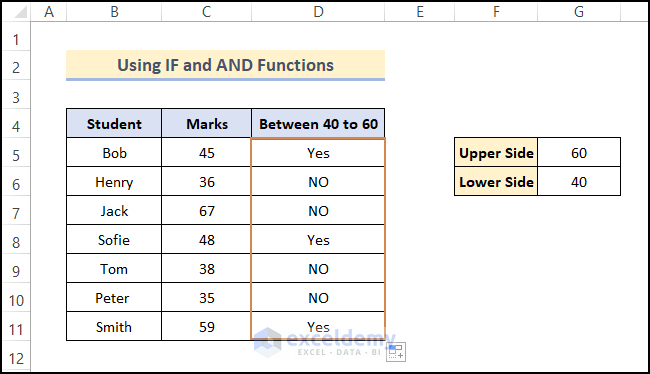
- Drag down the formula for other cells.
The result will look like below.
Read More: If a Value Lies Between Two Numbers Then Return Result in Excel
Method 4 – Using AND, MIN, and MAX Functions
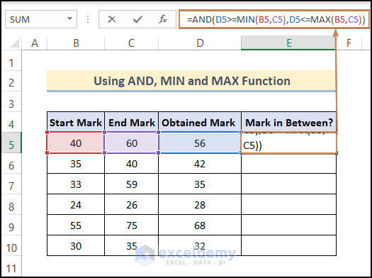
We can use the AND, MIN, and MAX functions to set a limit of a maximum value and minimum value range, then check if a value is between them.
Steps:
- Select cell E5 and enter the following formula:
=AND(D5>=MIN(B5,C5),D5<=MAX(B5,C5))
Here,
B5 = Start Mark.
C5 = End Mark.
D5 = Obtained Mark.
- Press ENTER.
Formula Breakdown:
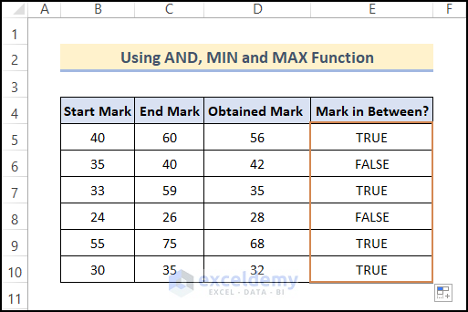
AND(D5>=MIN(B5,C5),D5<=MAX(B5,C5))→checks if the value of D5 is between the minimum value of B5 and C5 and the maximum value of B5 and C5. If the condition is met, it will return TRUE else FALSE.
- Drag down the formula to the rest of the cells with the Fill Handle.
Method 5 – Using Conditional Formatting to Highlight If a Value Is Between Two Numbers
The Conditional Formatting feature can be used to check if a value is between two numbers, then format the cells that match the condition with color to highlight them.
Steps:
- In cell D5 enter the following formula.
=AND(C5>=$G$7, C5<=$G$6)
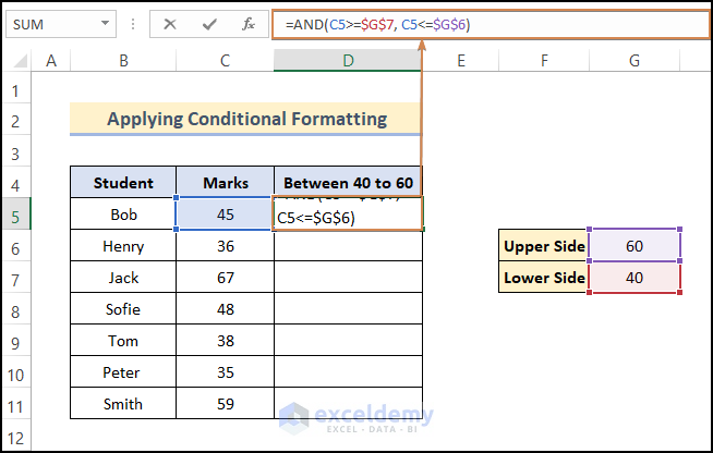
- Press ENTER.
- Drag down the Fill Handle to fill the other cells.
- Select the entire cell range D5:D11.
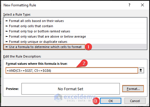
- Go to the Home tab >> click Conditional Formatting >> select New Rule.
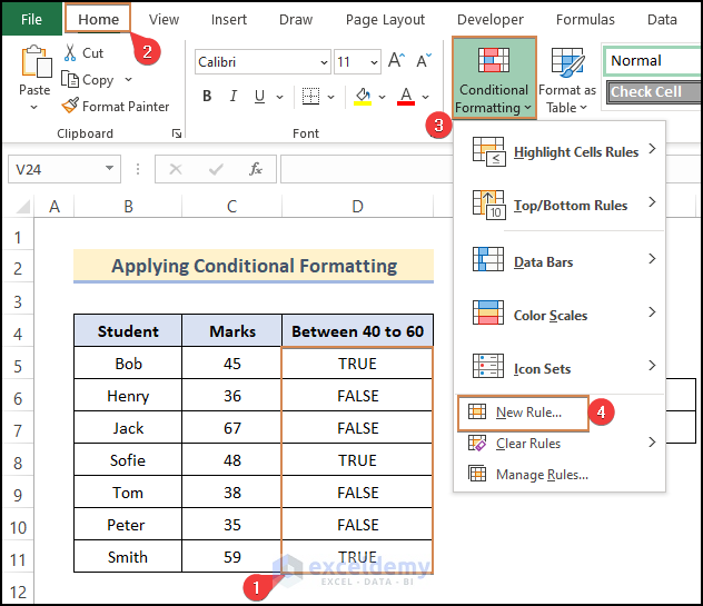
A dialog box will appear.
- Click Use a formula to determine which cells to format.
- In the Format values where this formula is true box, enter the above formula.
- Click Format.
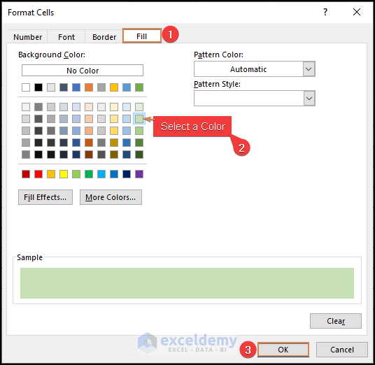
A new dialog wizard will open.
- Select Fill >> Select a color >> Click OK.
- Click Format.
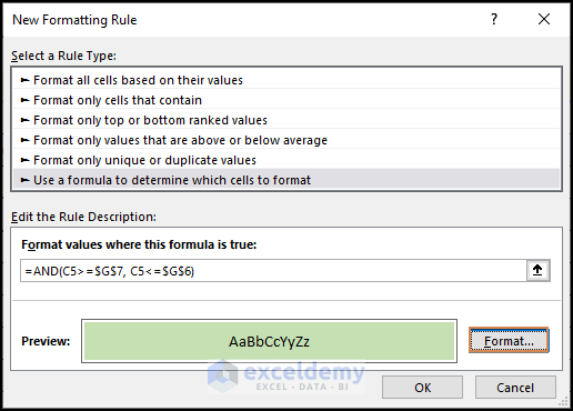
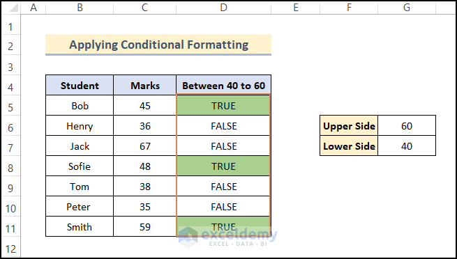
Our result will look like the screenshot below.
Download Practice Workbook
Check Value Between Two Numbers.xlsx
Related Articles
<< Go Back to Excel IF Function | Excel Functions | Learn Excel
Get FREE Advanced Excel Exercises with Solutions!

