Conditional Formatting Based on Multiple Values of Another Cell

Method 1 – Conditional Formatting on a Single Column Based on Multiple Values of Another Cell

Step 1: Select Column and Open Conditional Formatting

• Select the column on which you want to apply Conditional Formatting.
• Go to the Home > Conditional Formatting > New Rule option in Excel Toolbar.

We’ve selected column B (Product Name).

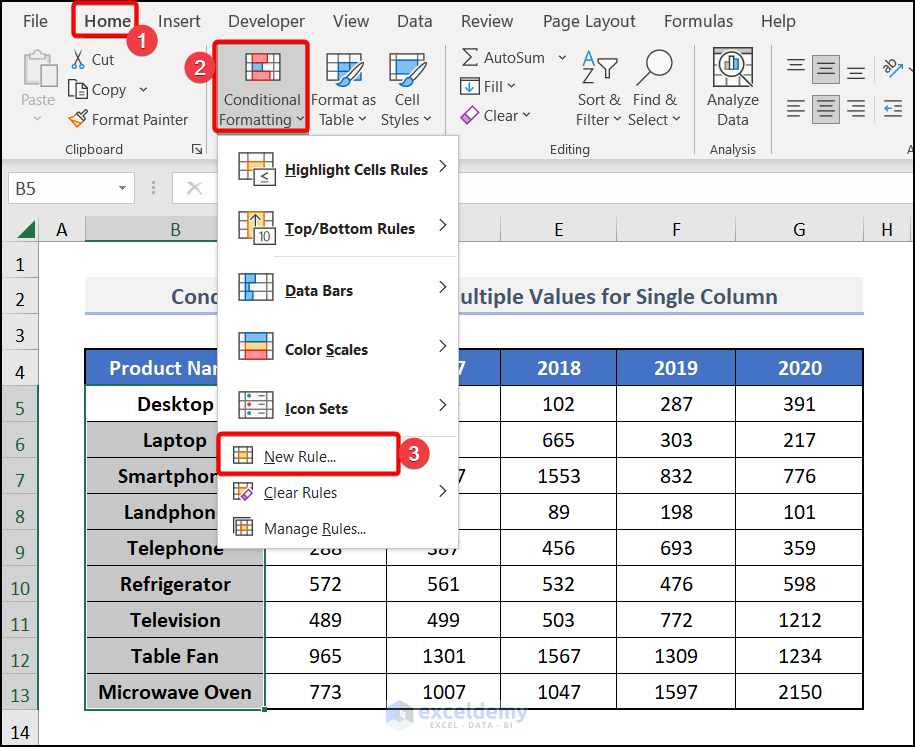
Step 2: Insert Formula in New Formatting Rule Box

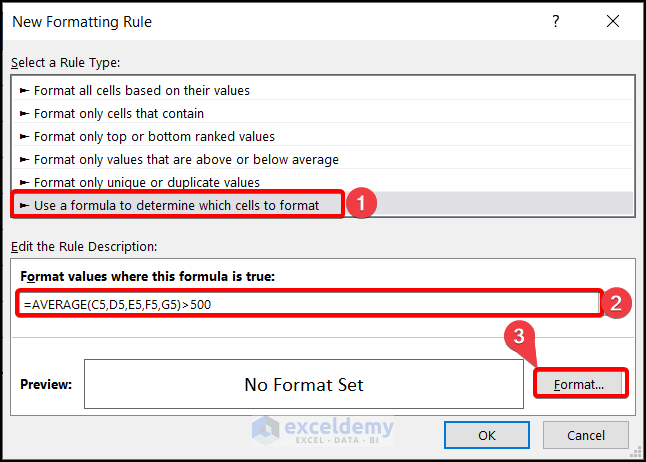
• Click on New Rule. A dialog box called New Formatting Rule will open.
• Click on Use a formula to determine which cells to format. Insert the following formula:

or

⧪ Notes:

• C5, D5, E5, F5, and G5 are the cell references of the first row, and AVERAGE()>500 is the condition.
• When applying Conditional Formatting on a single column based on multiple Values of another column, use either the Relative Cell References or the Mixed Cell References (Locking the Columns) of the cells, but not the Absolute Cell References.

Click on Format. You’ll be directed to the Format Cells dialogue box.

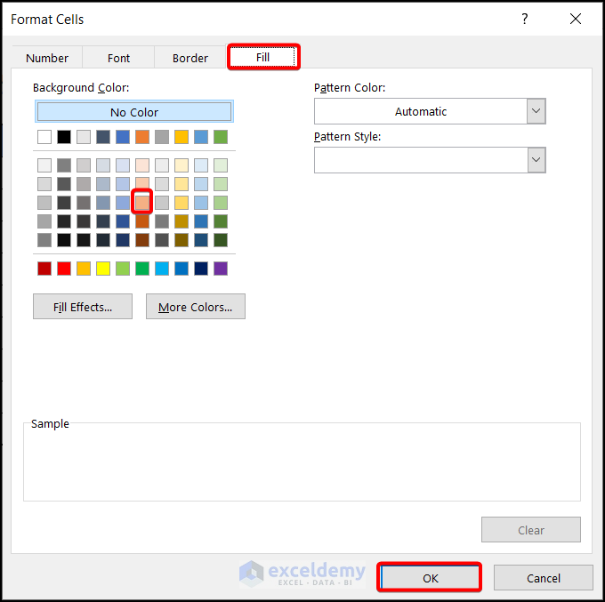
• From the formats available, choose the format you want to apply to the cells that fulfill the criteria.

We chose the light brown color from the Fill tab.

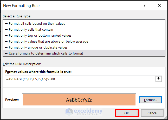
• Click on OK. You’ll be directed back to the New Formatting Rule dialog box.

Step 3: Final Output

• Click on OK.

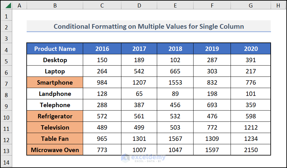
You’ll get the names of the products whose average sales are more than 500 marked in your desired format (Light brown in this example).

Read More: Conditional Formatting Based On Another Cell in Excel

Method 2 – Conditional Formatting on Multiple Columns Based on Multiple Values of Another Cell

The steps are the same as Example 1.

• Select all the columns on which you want to apply Conditional Formatting.

We have selected columns B, C, E and G.

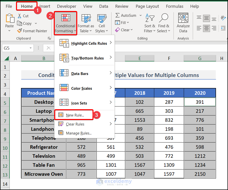
• Use the Mixed cell References (Locking the Columns) of the cells of the first row in the formula, not the Relative Cell References or the Absolute Cell References.

• Choose the desired format from the Format Cells Dialog Box. Click on OK twice.

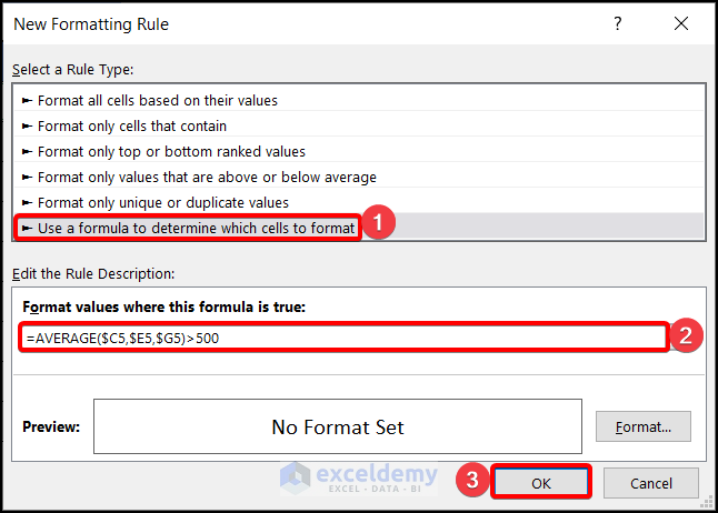
You will get the desired format applied to the cells of the multiple columns that fulfils your criteria.

⧪ More Examples:

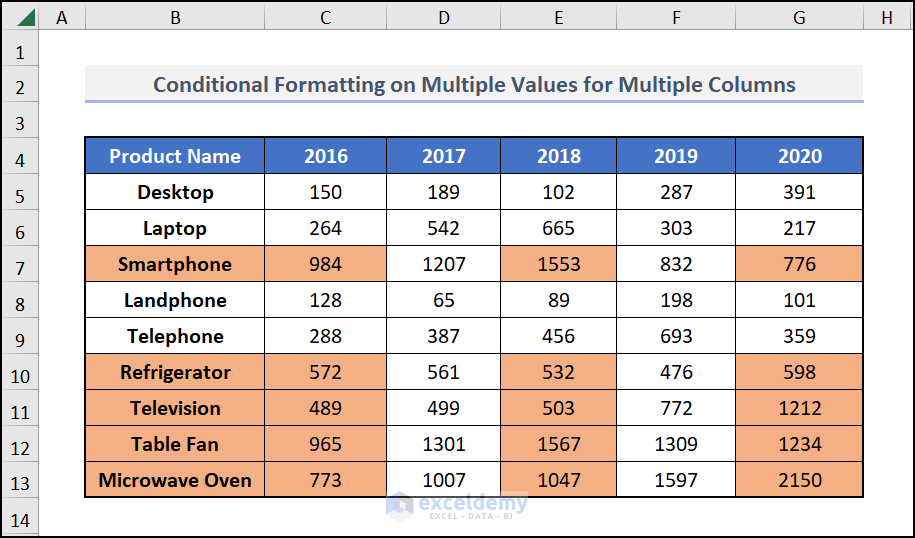
To apply Conditional Formatting to the whole data set, select the whole data set in step 1.

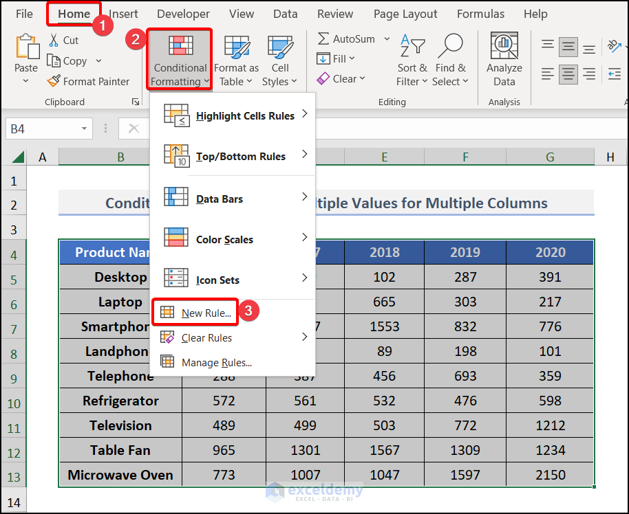
Apply the Mixed Cell References of the cells of the first row in the formula.

Select the desired format and hit OK.

You’ll get cells of the whole data set that fulfils the criteria marked in your desired format.

Read More: Conditional Formatting Entire Column Based on Another Column in Excel

Method 3 – Conditional Formatting on a Single Row Based on Multiple Values of Another Cell

Select the row on which you want to apply Conditional Formatting.

We’ve selected C4:G4 (Years).

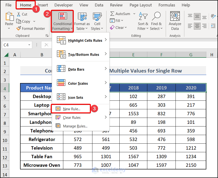
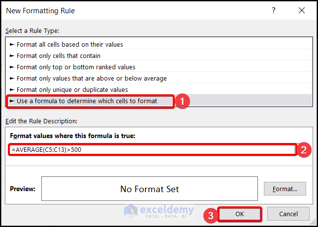
Use the Relative Cell References or the Mixed cell References (Locking the Rows) of the cells of the first column.

or

Choose the desired format from the Format Cells Dialog Box. Click on OK twice.

You will get the desired format applied to the years that had an average sales of more than 500.

Read More: Applying Conditional Formatting for Multiple Conditions in Excel

Method 4 – Conditional Formatting on Multiple Rows Based on Multiple Values of Another Cell

Select the rows on which you want to apply Conditional Formatting.

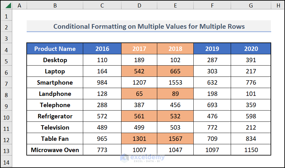
We’ve selected C4:G4, C6:G6, C8:G8, C10:G10, and C12:G12.

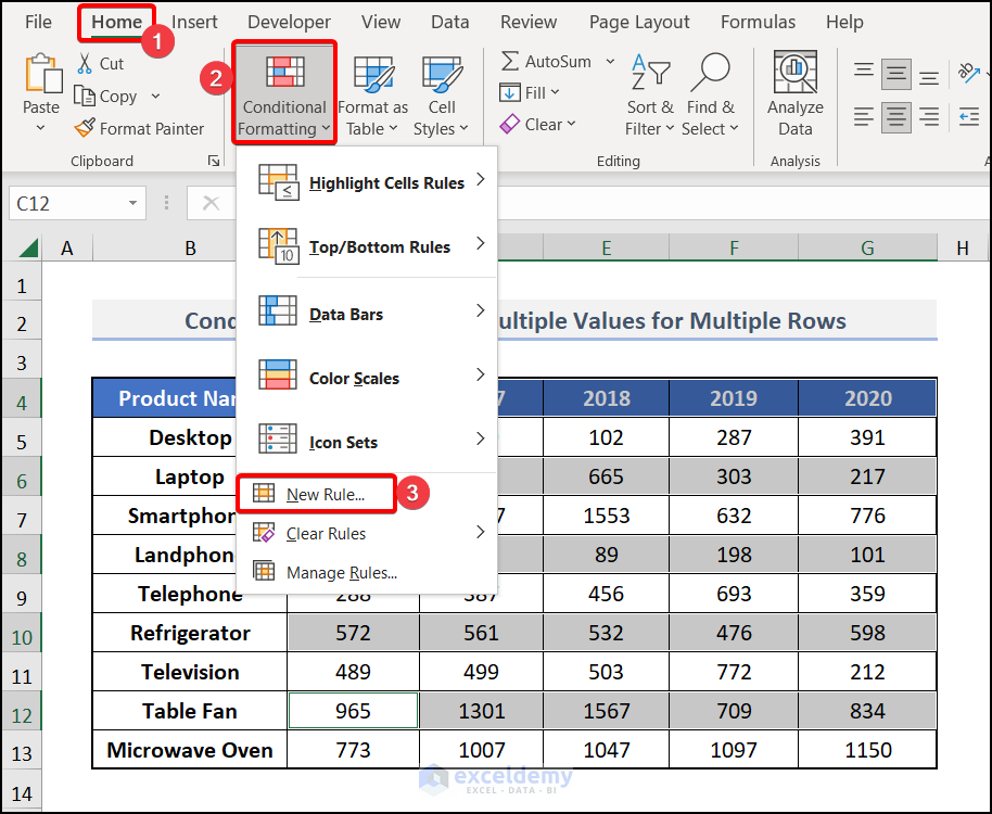
Use the Mixed cell References (Locking the Rows) of the cells of the first column in the formula.

Choose the desired format from the Format Cells Dialogue Box. Click on OK twice.

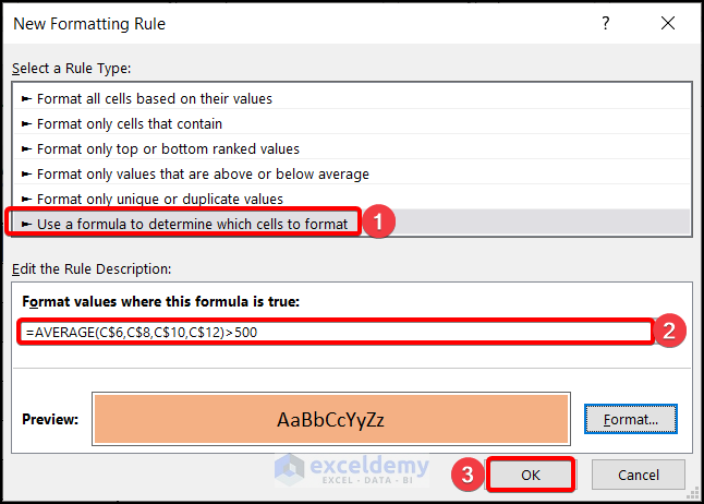
You will get the desired format applied to the cells that fulfils your condition.

Read More: How to Apply Conditional Formatting to Multiple Rows

How to Use Conditional Formatting with VBA Based on Another Cell

Steps:

• Navigate to the Developer tab >> choose Visual Basic.

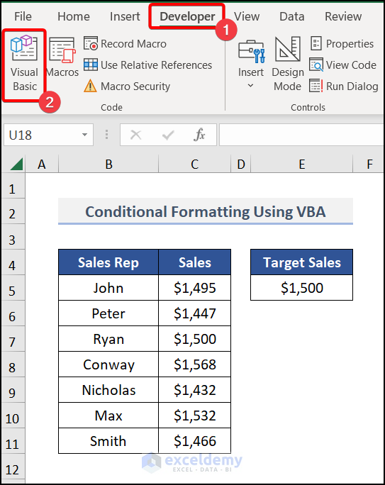
• Go to the Insert tab in the Visual Basic Editor >> Module >> Module 1.

• Enter the following code in Module 1.

Sub ConditionalFormatting()
Dim RG As Range
Dim CD1 As FormatCondition
Dim CD2 As FormatCondition
Dim CD3 As FormatCondition
Set RG = Range("C5", Range("C5").End(xlDown))
RG.FormatConditions.Delete
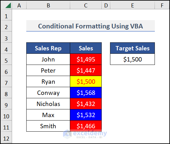
Set CD1 = RG.FormatConditions.Add(xlCellValue, xlGreater, "=$E$5")
Set CD2 = RG.FormatConditions.Add(xlCellValue, xlLess, "=$E$5")
Set CD3 = RG.FormatConditions.Add(xlCellValue, xlEqual, "=$E$5")
With CD1
.Interior.Color = vbBlue
.Font.Color = vbWhite
End With
With CD2
.Interior.Color = vbRed
.Font.Color = vbWhite
End With
With CD3
.Interior.Color = vbYellow
.Font.Color = vbRed
End With
End Sub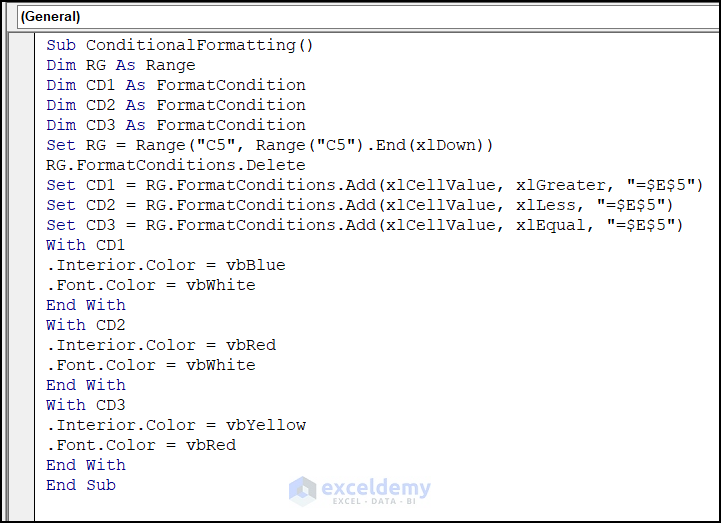

Press F5 to run the code and get the following result.

Download Practice Workbook

Related Articles

• Change Font Color Based on Value of Another Cell in Excel
• How to Apply Conditional Formatting to the Selected Cells in Excel
  
• Conditional Formatting Based On Another Cell Range in Excel

<< Go Back to Conditional Formatting with Multiple Conditions | Conditional Formatting | Learn Excel