How to Conditional Format for Dates Within 30 Days in Excel (3 Methods)

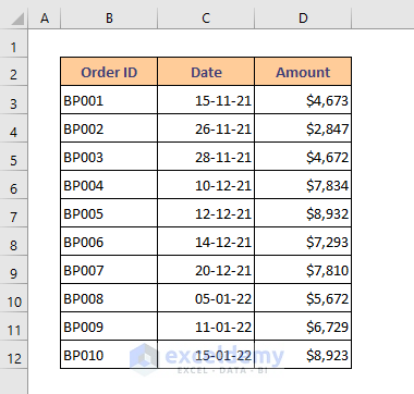
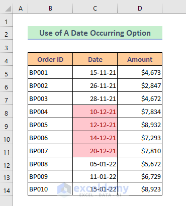
The below dataset has 3 columns displaying Order ID, Date, and Amount.

Method 1 – Conditional Formatting for Dates within 30 Days for Dates in a Range

Steps:

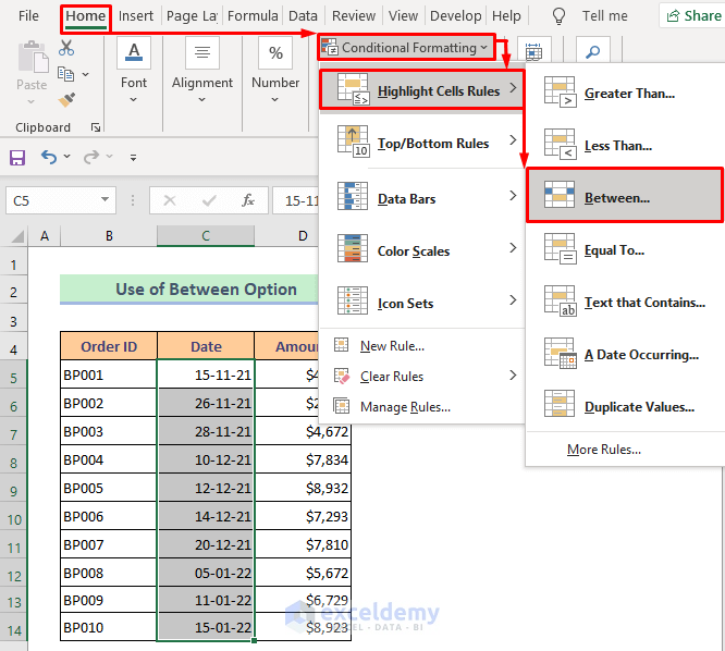
• Click: Home > Conditional Formatting > Highlight Cells Rules > Between

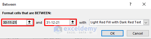
A dialog box will open up.

• Set a date range between 30 days. I have set 30-11-21 to 31-12-21.
• Press OK.

Now we have got our desired dates with highlighted colors.

Read more: Excel Conditional Formatting Based on Date

Method 2 – Conditional Formatting for Dates within 30 Days for a Specific Date

Steps:

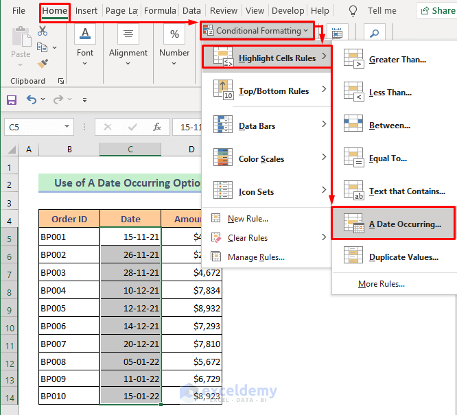
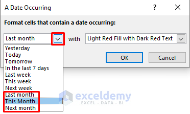
• Click: Home > Conditional Formatting > Highlight Cells Rules > A Date Occurring.

A dialog box will appear.

• Select your desired month from the date selection bar.
• Press OK.

Here’s the output for Last month.

And the output for This month.

And the output for Next month.

Read more: Apply Conditional Formatting to Overdue Dates in Excel

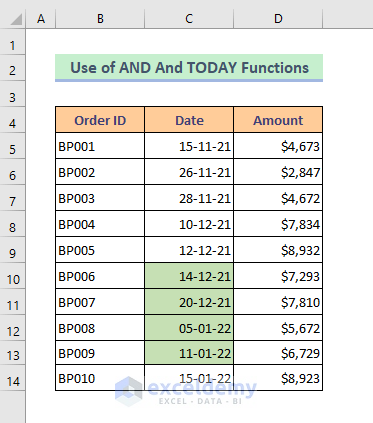
Case 3 – Combine AND and TODAY Functions with Conditional Formatting for Dates within 30 Days 

Steps:

• Click: Home > Conditional Formatting > New Rule.

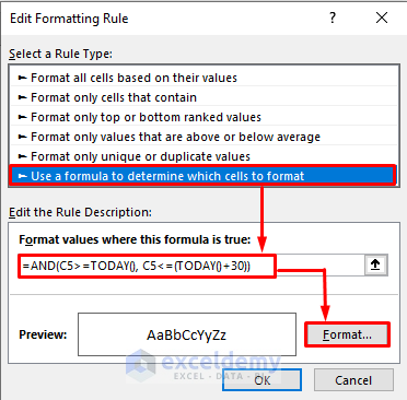
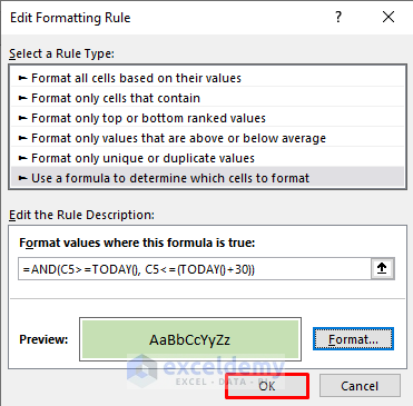
A dialog box named “Edit Formatting Rule” will open up.

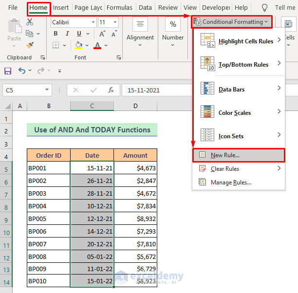
• Select Use a formula to determine which cells to format from Select a Rule Type bar.
• Enter the following formula in the Edit the Rule Description bar:

• Click Format.

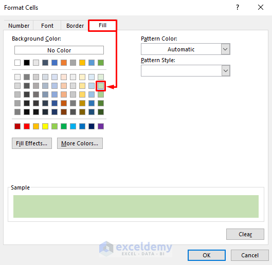
Format Cells dialog box will appear.

• Choose your desired color from the Fill option. I have chosen light green.
• Press OK, and we’ll go back to the previous dialog box.

• Press OK.

Now you will observe that the dates from today to the next 30 days are highlighted with our chosen light green color.

• For dates from today to the previous 30 days, enter the following formula:

How the formula works:

➥ C5>=TODAY()

Here, the TODAY function will check if the date in Cell C5 is greater than today’s date or not. So it returns:

FALSE

➥ C5<=(TODAY()+30)

It will check if the date is less than or equal to today’s date + 30 days and returns:

TRUE

➥ AND(C5<=TODAY(), C5>=(TODAY()-30))

The AND function encapsulates these two conditions. When both are true, the date is highlighted; otherwise, it is not highlighted.

Download the Practice Book

You can download the free Excel template from here and practice.

Related Articles

• Highlighting Row with Conditional Formatting Based on Date in Excel
• Conditional Formatting Based on Date in Another Cell in Excel
• Apply Conditional Formatting for Dates Older Than Today in Excel
• How to Change Cell Color Based on Date Using Excel Formula
• How to Apply Conditional Formatting to Each Row Individually
• How to Apply Conditional Formatting to Multiple Rows
• Conditional Formatting on Multiple Rows Independently in Excel
• How to Change Row Color Based on Text Value in Cell in Excel

<< Go Back to Conditional Formatting Based on Date | Conditional Formatting | Learn Excel