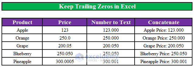
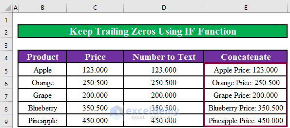
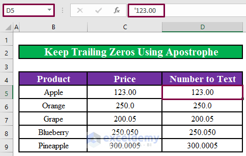
We have an Excel worksheet that contains information about different fruits and their price. We will use this worksheet to show how to convert number to text and keep trailing zeros in Excel. The image below shows the worksheet that we are going to work with.
Method 1 – Convert Numbers to Text and Keep Trailing Zeros in Excel Using the TEXT Function
Steps:
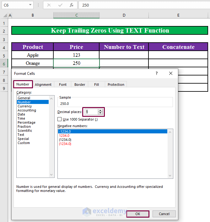
- Select a cell in the Price column to add decimal points to that cell value. We have selected cell C6.
- Right-click on that cell.
- Click on the Format Cells from the menu window.
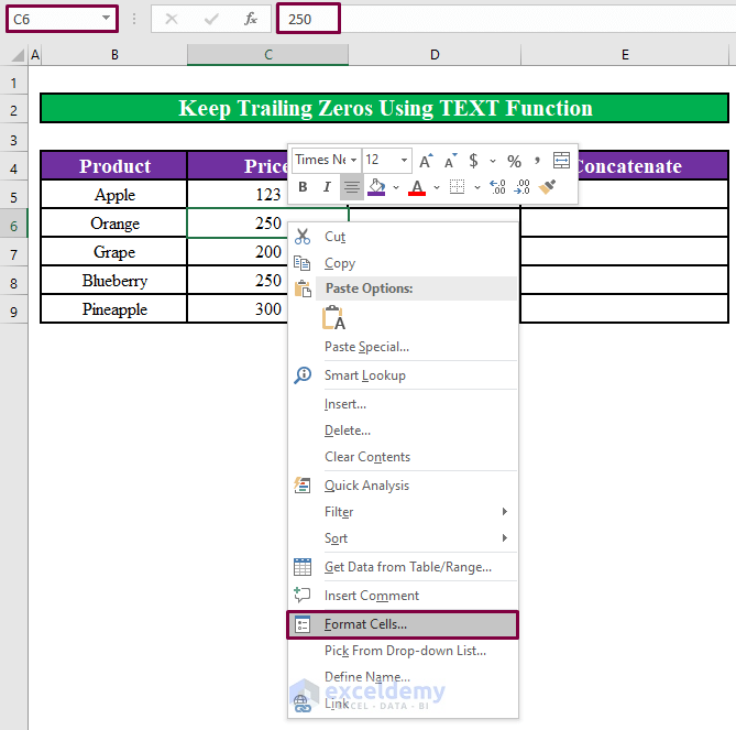
- A window titled Format Cells will appear. Set the Decimal Places to 1 to add a zero (0) after the decimal place.
- Click on OK.
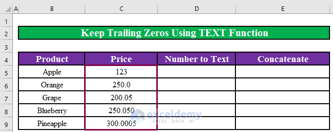
- Increase the decimal places to different numbers for different values of the Price.
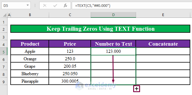
- Use the following formula in cell D5.
=TEXT(C5,"##0.000")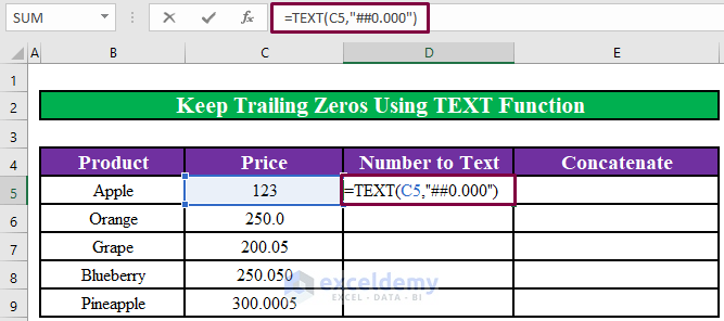
Formula Breakdown:
Using the TEXT function, you can apply formatting to a number with format codes to change the way it appears.
- The number in cell C5 has been converted to text with the trailing zeros following the decimal point.
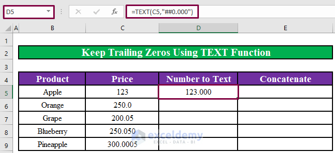
- Drag the fill handle of cell D5 to apply the formula to the rest of the cells.
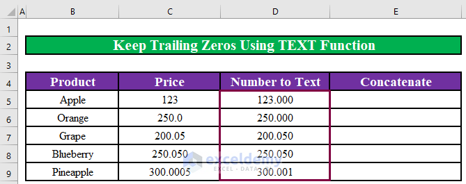
- All the numbers in the Price column have been converted to text with the trailing zeros following the decimal point.
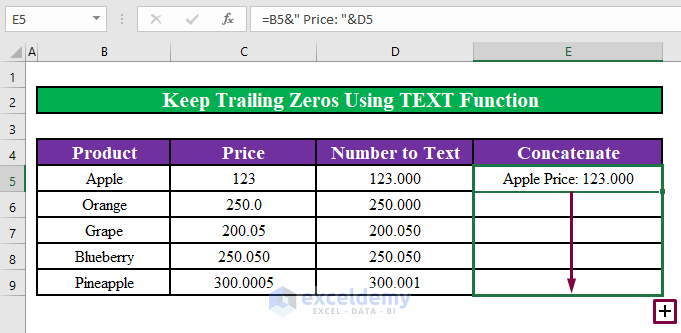
- Insert the following formula in cell E5.
=B5&" Price: "&D5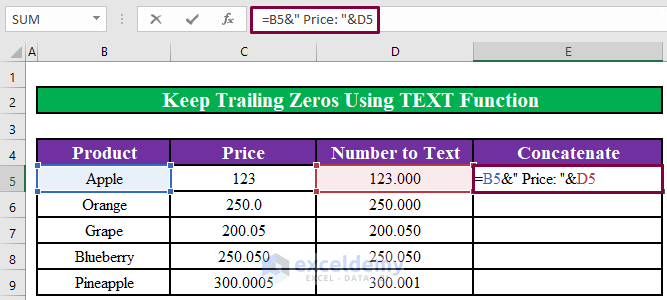
Formula Breakdown:
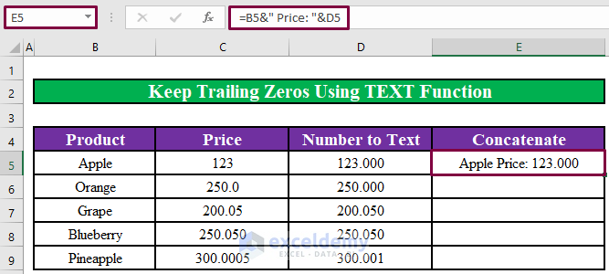
The Ampersand sign (&) will concatenate the texts in cells B5 and D5 with the text “Price“ between the two texts.
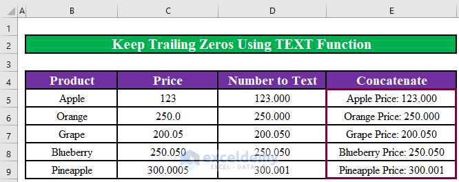
- Texts in cells B5 and D5 have been concatenated using the ampersand (&) sign.
- Drag the fill handle of cell E5 to apply the formula to the rest of the cells.
- Here’s the result.
Read More: How to Convert Number to Text with Leading Zeros in Excel
Method 2 – Use the IF Function to Convert Numbers to Text and Keep Trailing Zeros in Excel
Steps:
- Add decimal points to the cell values in the Price column as in Method 1.
- Use the following formula in cell D5.
=IF(CELL("FORMAT",C5)="F3", TEXT(C5,"0.000"), TEXT(C5, 0))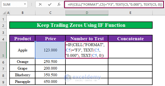
Formula Breakdown:
- IF function will check if the number has 3 decimal points.
- If the number has 3 decimal points, the TEXT function will convert the number to text while keeping those 3 decimal points with the number.
- If the number does not have 3 decimal points, the TEXT function will convert the number to text without changing anything.
- The number in cell C5 has been converted to text with the trailing zeros following the decimal point.
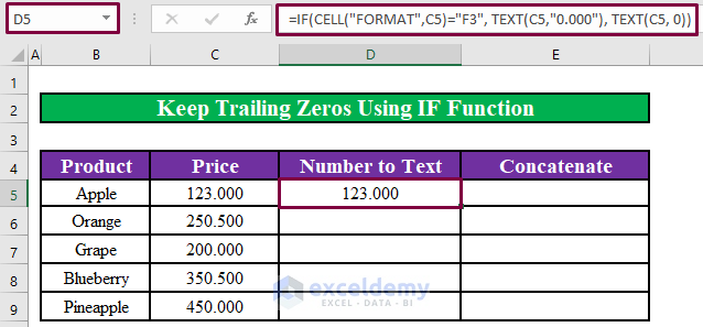
- Drag the fill handle of cell D5 to apply the formula to the rest of the cells.
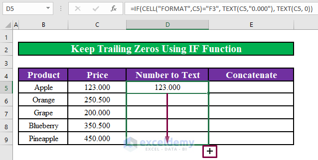
- All the numbers in the Price column have been converted to text with the trailing zeros following the decimal point.
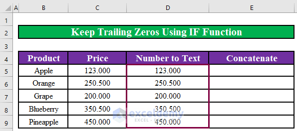
- If we use the same concatenation formula using the ampersand (&) sign, we will see that respective texts in the Product and Number to Text columns have been concatenated.
Method 3 – Convert Numbers to Text and Keep Trailing Zeros Using the Apostrophe Symbol
Steps:
- Put an apostrophe sign (‘) in front of each number in the Price column. That will convert the number to text while keeping trailing zeros.
Read More: How to Convert Number to Text with Commas in Excel
Method 4 – Use VBA Code to Convert Numbers to Text and Keep Trailing Zeros in Excel
Steps:
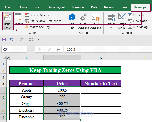
- Select all the cells in the Price column.
- Select Visual Basic from the Developer tab. You can also press Alt + F11.
- Click on the Insert button and select Module.
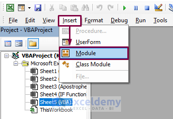
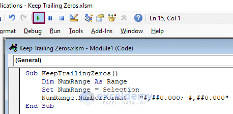
- Insert the following code in the window that appears.
Sub KeepTrailingZeros()
    Dim NumRange As Range
    Set NumRange = Selection
    NumRange.NumberFormat = "#,##0.000;-#,##0.000"
End Sub- Click on the Run (▶).
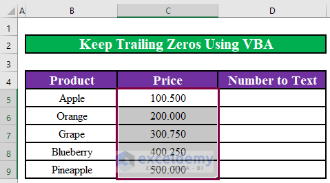
- All the numbers in the Price column have been converted to text with the trailing zeros following the decimal point.
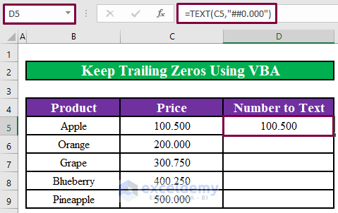
- Use the same TEXT formula we have used in Method 1 in cell D5 to convert the number in cell C5 to text.
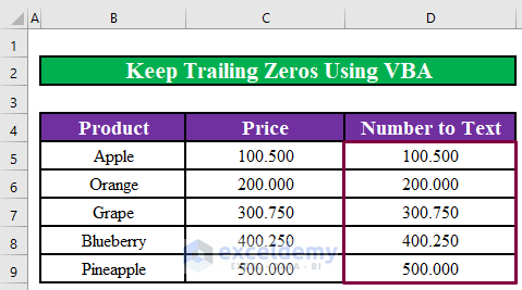
- Upon dragging the fill handle downward to apply the formula to the rest of the cells, we will see that all the numbers in the Price column have been converted to text with the trailing zeros following the decimal point.
Bonus – Add Trailing Zeros Using a Formula in Excel
Steps:
- Use the following formula in cell D5.
=C5&REPT("0",5-LEN(C5))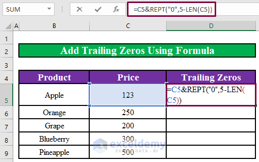
Formula Breakdown:
- LEN(C5) will measure the length of the value in cell C5. The function will return 3 as the value in C5 is a 3 digits number.
- 5-LEN(C5) will be 2.
- The REPT function will then repeat the number zero (0) 2 times.
- The ampersand (&) sign will then concatenate the value of cell C5 and the two zero (0) together to add two trailing zeros after the number in cell C5.
- The number in cell C5 has two trailing zeros.
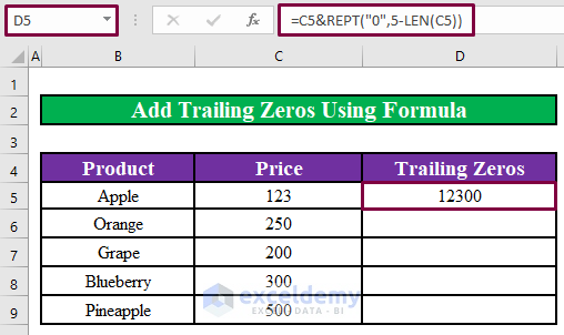
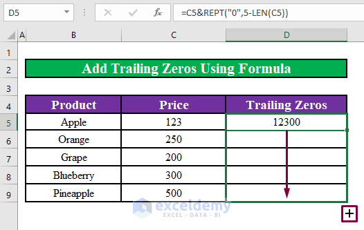
- Drag the Fill handle of cell D5 to apply the formula to the rest of the cells.
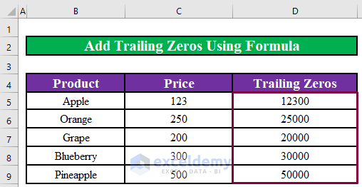
- The formula has added two trailing zeros to each number in the Price.
Quick Notes
- If you do not have the Developer tab, you can make it visible via File > Option > Customize Ribbon.
Download the Practice Workbook
Related Articles
- How to Convert Number to Text in Excel with Apostrophe
- How to Convert Number to Text with Green Triangle in Excel
- Convert Number to Text without Scientific Notation in Excel
- How to Convert Number to Text with 2 Decimal Places in Excel
- How to Convert Number to Text for VLOOKUP in Excel
<< Go Back to Excel Convert Number to Text | Learn Excel
Get FREE Advanced Excel Exercises with Solutions!
