How to Convert Number to Text without Scientific Notation in Excel

In Excel, if you input a number with 15 or more digits, although the number is stored in number format as usual, it is displayed by default in scientific notation. In some specific cases, we may need to convert these numbers to text excluding the scientific notation, in order to search the data part by part, match two cells, better visualize the values, etc.

In this article, we will describe 7 methods to convert any number to text without scientific notation in Excel.

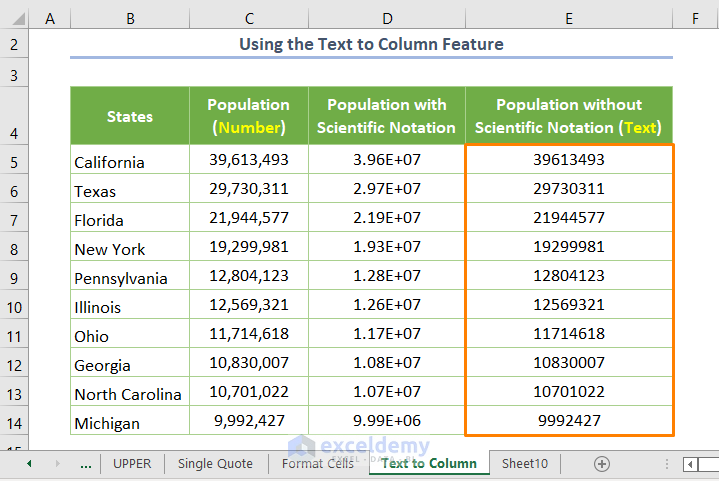
In the following dataset, the population of the top 10 most populated states is provided in the range C5:C14 in number format. Expressed in scientific notation using the Format Cells option, it looks like the range D5:D14.

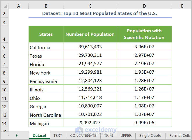
Let’s convert the numbers to text without scientific notation.

Method 1 – Using the TEXT Function

The TEXT function converts a value to text in a specified format.

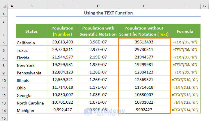
Insert the following formula in cell E5:

=TEXT(D5,"0")

Here, D5 is the starting cell of the population with scientific notation, and 0 is the format code that shows all insignificant zeros. That’s why the output will act as text.

After inserting the formula, press ENTER and drag down the plus sign located at the lower-right corner of the E5 cell (Fill Handle Tool) to get the output (E5:E14 cell range).

Method 2 – Using the CONCATENATE Function

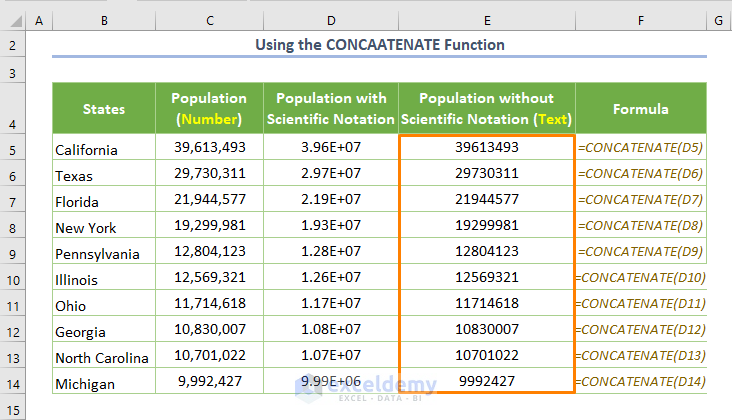
We can accomplish the same task using the CONCATENATE function, which combines multiple strings into a single string.

So, the formula will be:

=CONCATENATE(D5)

Method 3 – Using the TRIM Function

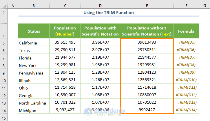
Similarly, the TRIM function will provide us with the same output, because it stores numbers in text format and removes unnecessary spaces from the text string.

The adjusted formula is:

=TRIM(D5)

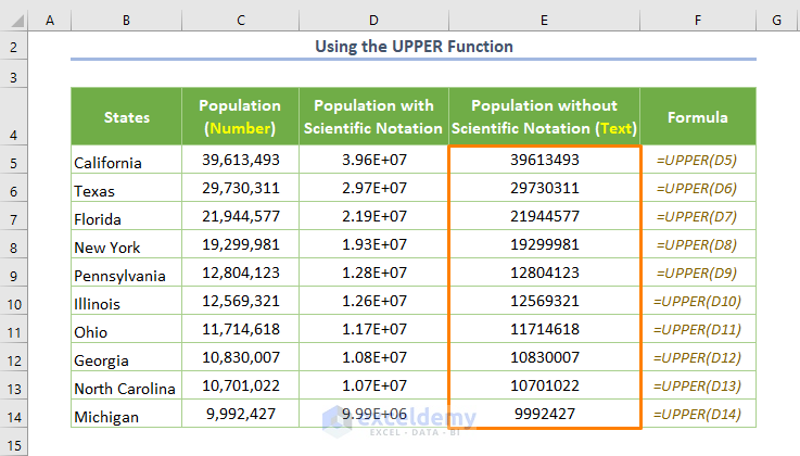
Method 4 – Using the UPPER Function

The UPPER function mainly converts a text string to all uppercase letters. But we can use it here, as it will store any number entered as input in text format.

The formula will be:

=UPPER(D5)

Method 5 – Adding a Single Quote

There are other methods to convert numbers to text besides using Excel functions. Simply adding a Single Quote or Apostrophe (‘) before the number will convert it to text. So, input the following in the corresponding formula bar:

'Any number that you want to convert

If we take the example of cell D5, insert:

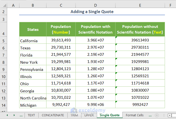
'39613493

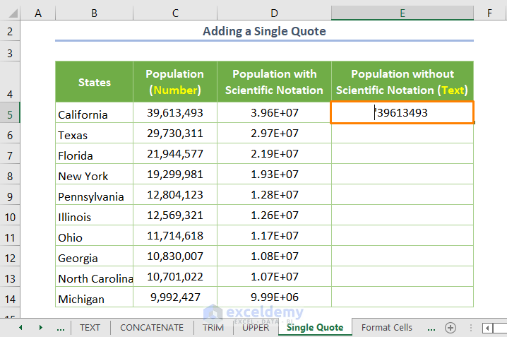
If you now press ENTER, the output will be returned but with a green triangle in the upper-left corner showing an error in the cell.

To remove the error, click on the triangle and choose the Ignore Error option.

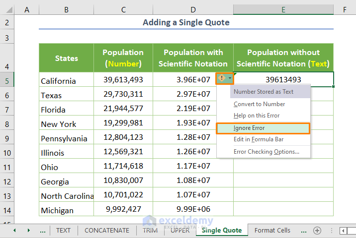
Now the number is in text format without an error. We could repeat the same process for the rest of the cells, i.e. manually adding a single quote and inserting the number. Obviously, that’ll be a tedious and time-consuming task. Fortunately, we can use the Flash Fill tool instead to apply the same format to the cells below.

Insert a single quote in cell E6, and you’ll automatically see the preview to fill (or press CTRL + E to turn on the tool).

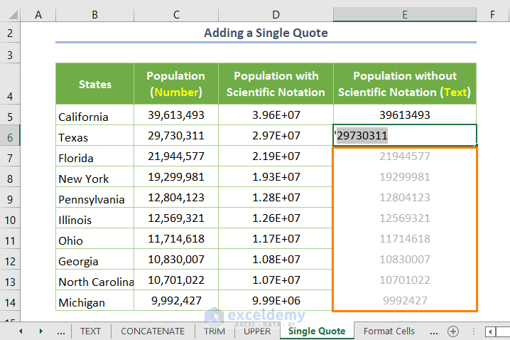
Click on the last cell of the preview (cell E14)

The following is the output:

Method 6 – Using the Format Cells Option

We can also apply the Format Cells option to quickly convert numbers to text.

Steps:

Copy the range D5:D14 by pressing CTRL + C, and paste the copied cells in cell E5 by pressing CTRL + V.

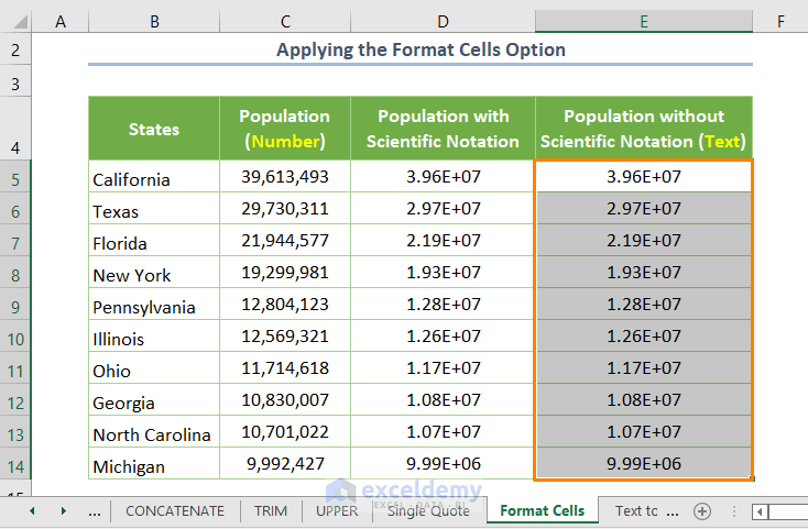
Select the range E5:E14.
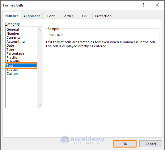
Open the Format Cells option by pressing the CTRL + 1 keyboard shortcut.
Choose the Text option from the Number tab in the dialog box.
Click OK.

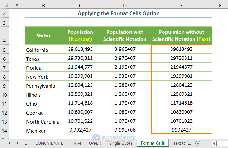
The desired output in text format is returned.

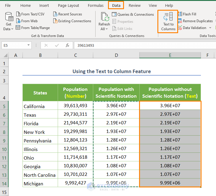
Method 7 – Using the Text to Column Feature

Lastly, we can use the Text to Columns feature to convert the numbers to text as well as remove the scientific notation.

Steps:

Copy the data and paste it into the E5:E14 cell range.
With the data selected, click on the Text to Column feature from the Data Tools ribbon in the Data tab.

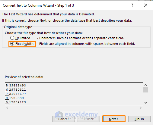
In the dialog box that opens, select Fixed Width.
Click on the Next button.

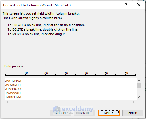
Again, click on the Next button.

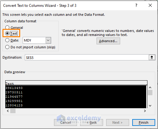
In Step 3 of 3, check the circle before the Text format.
Click on Finish.

The following output is returned.

Quick Notes

To check whether your converted output is in text format or not, apply the ISTEXT function as follows:

=ISTEXT(D5)

The ISTEXT function returns TRUE if it finds text in the cell, else it returns FALSE.

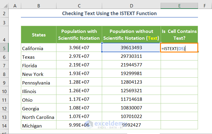
After pressing ENTER and using the Fill Handle Tool, the output will look like the following:

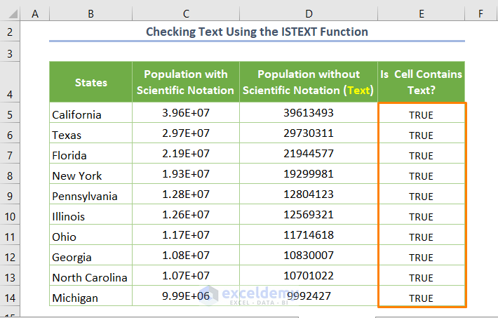
The output is clearly in text format.

Note: Here, I took the output found using the TEXT function as an example. You may check the output for the rest of the methods at your leisure.

In this dataset, we converted the number with scientific notation manually for purpose of demonstration. However, the input number will be automatically stored with a scientific notation if the number is very large or very small. For example, the maximum limit of precision is 15 in the case of Number format, and 12 in the case of General format.
Also, using the above methods you may add leading zeros before the output which is in the Text format.

Download Practice Workbook

Converting Number to Text without Scientific Notation.xlsx

<< Go Back to Excel Convert Number to Text | Learn Excel

Get FREE Advanced Excel Exercises with Solutions!