Let’s use the following dataset, which contains some Subject and Marks. The numbers are showing errors (or error suggestions) because the format is not a number.

Method 1 – Converting an Entire Column to Numbers in Excel with the Convert to Number Option
In this scenario, the error is showing because there is an Apostrophe before the number.
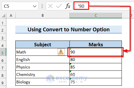
Steps:
- Select the data of the column where the error is showing.
- Select the warning sign.
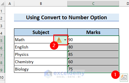
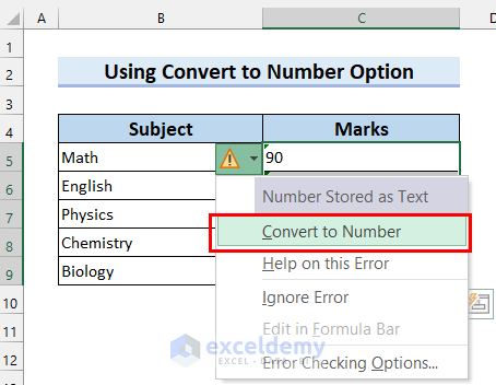
- A drop-down menu will appear.
- Select Convert to Number.
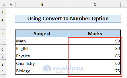
- The entire column has been converted to numbers.
Method 2 – Convert to Number by Multiplying
Steps:
- Add a Helper Column in the dataset.

- Select the cell where you want to convert to number. We selected cell D5.
- Insert the following formula:
=C5*1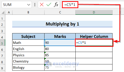
- Press Enter to convert to number.
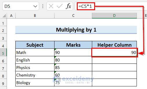
- Drag the Fill Handle down to copy the formula.
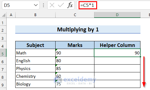
- The formula is copied to the entire column.
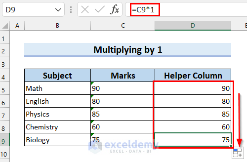
- The entire column has been converted to numbers.

Read More: How Excel Formulas Convert Text to Number
Method 3 – Adding 0 to Convert an Entire Column to Numbers in Excel
Steps:
- Add a Helper Column in your dataset.
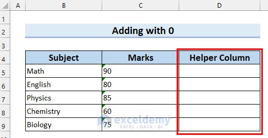
- Select the cell where you want to convert to number. We selected cell D5.
- Insert the following formula:
=0+C5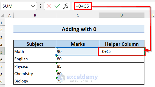
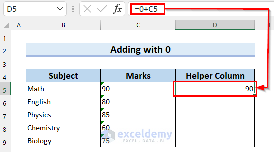
- Press Enter to convert to number.
- Drag the Fill Handle down to copy the formula.
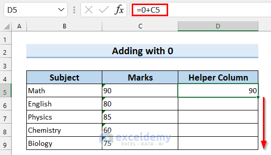
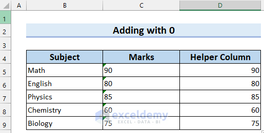
- We have copied the formula to the entire column.
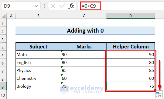
- The entire column has been converted to numbers.
Read More: How to Convert Text with Spaces to Number in Excel
Method 4 – Performing Division to Convert an Entire Column to Number
Steps:
- Add a Helper Column D in your dataset.

- In cell D5, insert the following formula:
=C5/1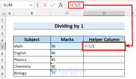
- Hit Enter.
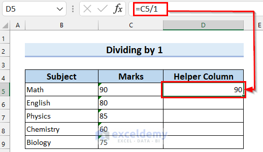
- Drag the Fill Handle down to copy the formula.
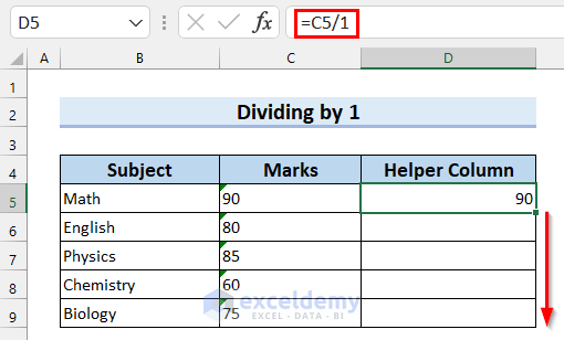
- This copies the formula to the entire column.
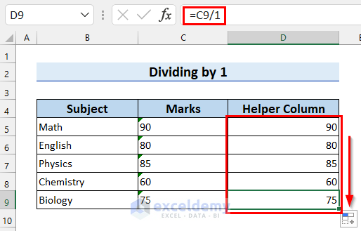
- You can check the results below.

Method 5 – Changing the Cell Format in Excel to Convert an Entire Column to Numbers
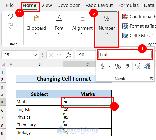
- Select the cell where the error is showing.
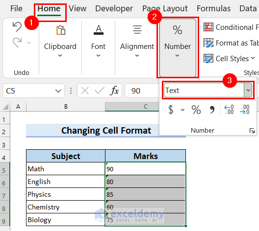
- Go to the Home tab.
- Select Number.
- Check the Cell Format. Here, you can see that it is selected as Text.
- Select the entire data range.
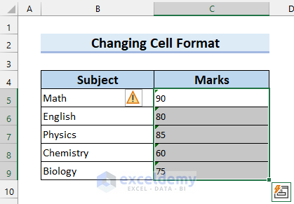
- Go to the Home tab from the Ribbon.
- Select Number.
- Select the drop-down option on the selected Cell Format.
- Select General or Number. We selected General.
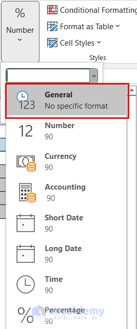
- This should convert the entire column to numbers if the values are only numbers.

Method 6 – Using the Excel Paste Special Option to Convert an Entire Column to Numbers
Steps:
- Copy an empty cell that is not in Text format. We copied cell B11.

- Select the data where the error is showing.

- Right-click on the selected column.
- Select Paste Special.

- A dialog box named Paste Special will appear.
- Select All from Paste.
- Select Add from Operation.
- Select OK.

- This will convert the entire column to numbers.

Method 7 – Using Text to Columns Feature for Converting an Entire Column to Number
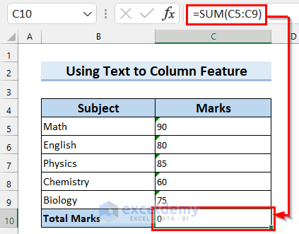
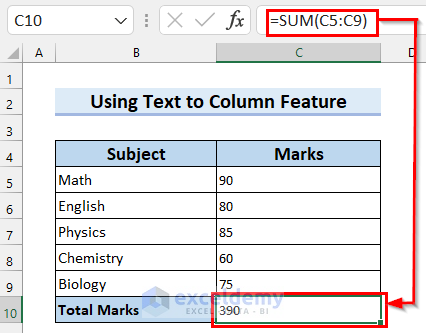
In the following picture we can see that the SUM function is not working. That means the numbers here are stored as Text.
Steps:
- Select the data where the error is showing.
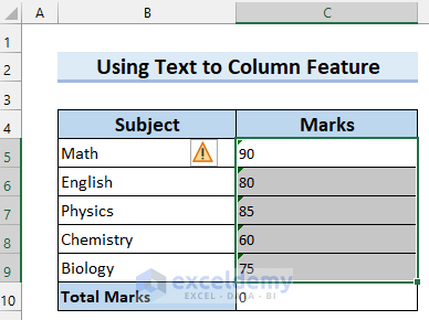
- Go to Data tab.
- Select Text to Columns from Data Tools.

- The Convert Text to Columns Wizard will appear on the screen.
- Select Delimited from the Original data type.
- Press Next.
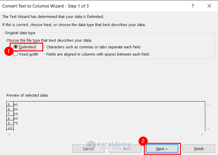
- Step 2 of Convert Text to Columns Wizard will appear.
- Select Tab from Delimiters.
- Select Next.
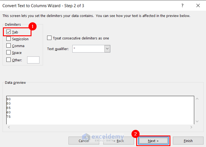
- Step 3 of Convert Text to Columns Wizard will appear.
- Select General in Column data format.
- Select the 1st cell of your column as Destination.
- Press Next.
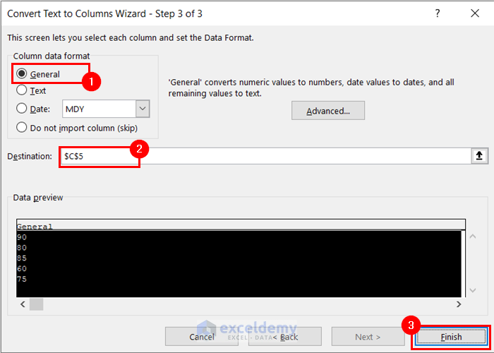
- This will convert the entire column to numbers.
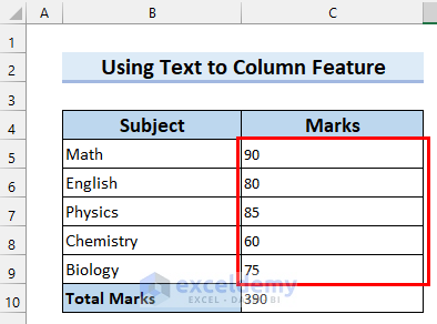
- The numbers will keep their alignment to the left (Excel usually aligns numbers to the right), but the formulas work.
 Read More: How to Convert Bulk Text to Number in Excel
Method 8 – Use the VALUE Function to Convert an Entire Column to Numbers
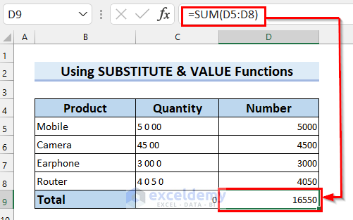
If you enter numbers with extra spaces, they will be stored as text.
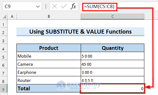
Steps:
- Add a new column to your dataset that will store numbers.
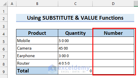
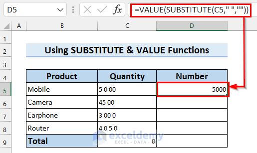
- Select the cell where you want to convert the first number. We selected cell D5.
- Insert the following formula:
=VALUE(SUBSTITUTE(C5," ",""))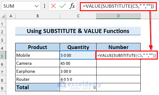
Formula Breakdown
- SUBSTITUTE(C5,” “,””): The SUBSTITUTE function will replace the extra spaces with no space.
- Output: “5000”
- VALUE(SUBSTITUTE(C5,” “,””)): turns into
- VALUE( “5000”)—-> The VALUE function will convert the text format into a number format.
- Output: 5000
- Explanation: We got the result 5000 as a numeric value.
- VALUE( “5000”)—-> The VALUE function will convert the text format into a number format.
- Press Enter to get the result.
- Drag the Fill Handle to copy the formula.
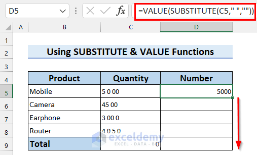
- This fills in the column with the formula.
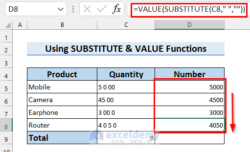
- In cell D9, insert the following formula:
=SUM(D5:D8)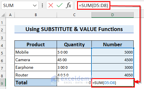
- Press Enter to get the sum.
Method 9 – Converting the Entire Column to Numbers with Excel Power Query
Steps:
- Copy your dataset.
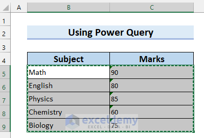
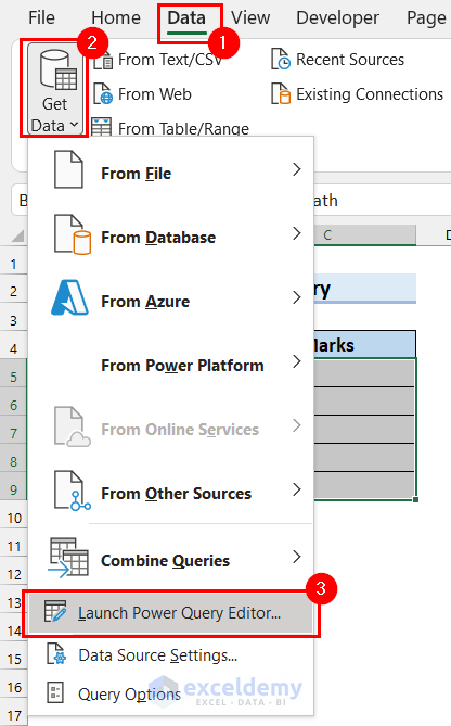
- Go to the Data tab.
- Select Get Data.
- A drop-down menu will appear.
- Select Launch Power Query Editor.
- The Power Query Editor will appear.
- Go to the Home tab.
- Select Enter Data.

- The Create Table option will appear.

- Right-click on the first cell.
- Select Paste.

- Select Undo Headers.

- Select OK.
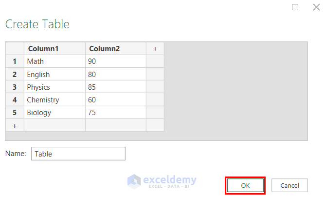
This imports the dataset to Power Query. Here, you can see that the format is automatically converted to number.
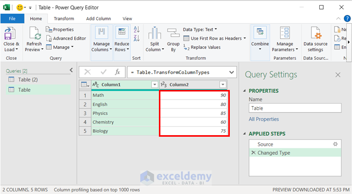
- Click on the marked portion in the image.
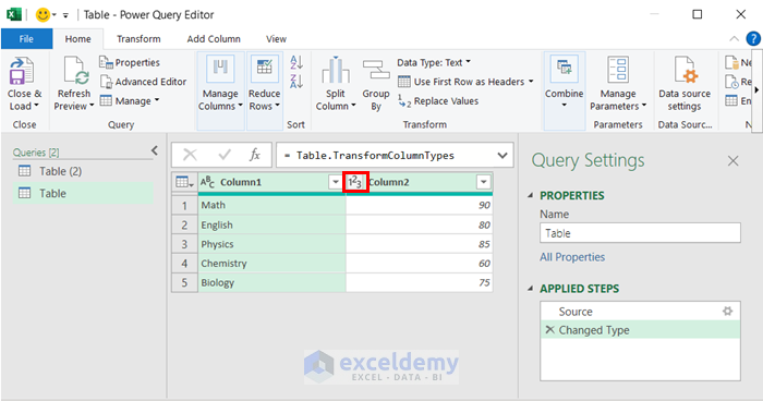
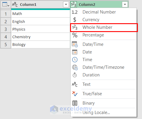
- You will see a drop-down menu.
- Select Whole Number.
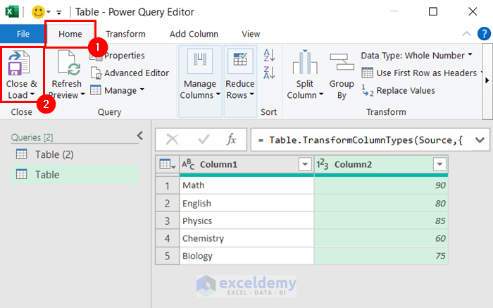
- Go to Home tab.
- Select Close & Load.
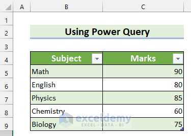
- You will get the table in your worksheet.
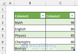
- You can change the font size and edit the table as you want.
Download the Practice Workbook
Related Articles
- How to Convert Alphabet to Number in Excel
- How to Fix Convert to Number Error in Excel
- How to Fix All Number Stored as Text in Excel
<< Go Back to Convert Text to Number in Excel | Learn Excel
Get FREE Advanced Excel Exercises with Solutions!

