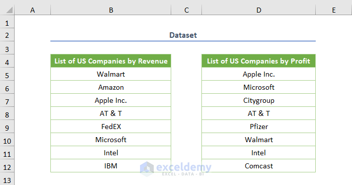
Column B depicts the List of US Companies by Revenue (List-1) while column D shows the List of US Companies by Profit (List-2). We’ll count the number of duplicates across two columns.
Method 1 – Count Duplicates in Two Columns Using the COUNTIF Function
The generic formula is:
=COUNTIF(Range, Criteria)
- Use the following formula:
=COUNTIF($B$5:$D$12, B5)
$B$5:$D$12 is the range where I want to count duplicates, and B5 is the specific cell that I want to count (criteria).
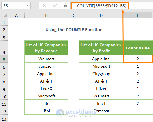
- The value of duplicates is 2 or higher. The value of unique records is 1.
- We can wrap the logical IF function to return Duplicates instead of getting a number:
=IF(COUNTIF($B$5:$D$12,B5)>1, "Duplicates","Unique")
If the value of the syntax COUNTIF($B$5:$D$12,B5) is greater than 1, the above formula will return Duplicates. Otherwise, it’ll return Unique.
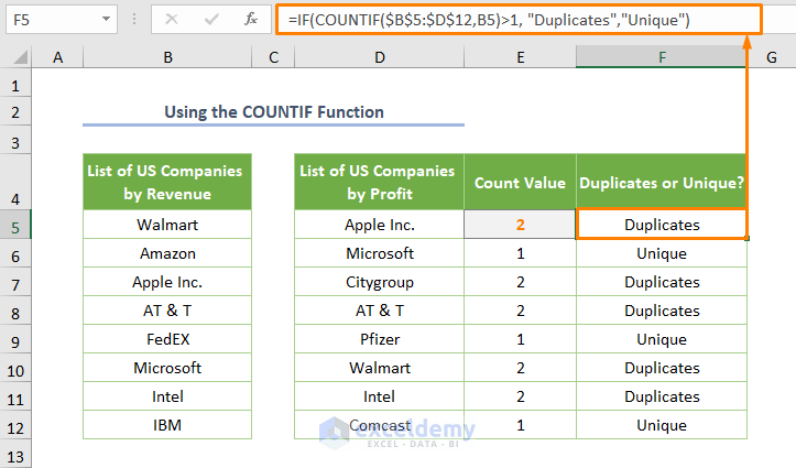
Note that this formula only checks the values from one column, but counts their occurrences in both.
Read More: How to Count Duplicates in Column in Excel
Method 2 – Count Duplicates in Two Columns Using the SUMPRODUCT and COUNTIF Functions
- Use the following formula:
=SUMPRODUCT(COUNTIF($B$5:$B$12,$D$5:$D$12))
$B$5:$B$12 is the cell range representing the list of companies by revenue (List-1), and $D$5:$D$12 is the cell range depicting the list of companies by profit (List-2).
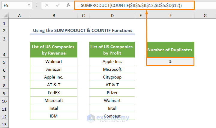
The COUNTIF function counts the number of duplicates separately. The function returns 1 for the first row as depicted in the following image.
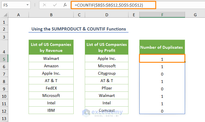
The SUMPRODUCT function sums up the values that were found using the COUNTIF function.
Read More: How to Count Duplicate Values in Multiple Columns in Excel
Method 3 – Utilizing the Combination of SUMPRODUCT and MATCH
- The combined formula for the F5 cell is as follows:
=SUMPRODUCT(--(ISNUMBER(MATCH(B5:B12,D5:D12,0))))
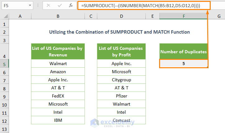
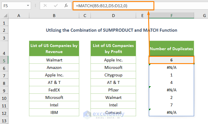
The MATCH function returns the relative position of matched values. The function returns #N/A when there exist unique records as shown in the following screenshot. The ISNUMBER function is used to return TRUE or FALSE to avoid #N/A.
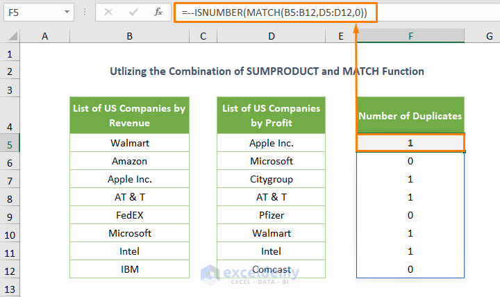
We used a double dash (—) before the ISNUMBER function to convert TRUE or FALSE (boolean values) into integer values.
The SUMPRODUCT sums up all values and returns 5 which is the number of duplicates.
Read More: Count Number of Occurrences of Each Value in a Column in Excel
Method 4 – Applying the Excel SUM and MATCH Functions to Count Duplicates in Two Columns
- Use the following formula:
=SUM(IF(ISNA(MATCH(B5:B12,D5:D12,0)),0,1))
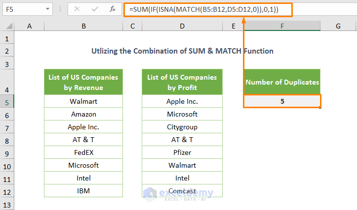
The ISNA function omits the #N/A error found by the MATCH function. It returns TRUE for duplicate values and FALSE for unique values.
We assigned the logical IF function to get 1 for the TRUE boolean value and 0 for the FALSE value.
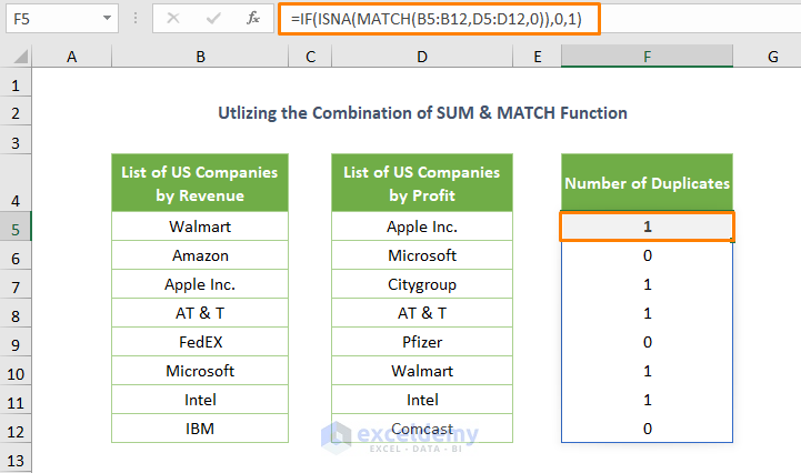
The SUM function will return the number of duplicate values.
Read More: Count the Order of Occurrence of Duplicates in Excel
Method 5 – Counting Duplicates in Two Columns Using the VLOOKUP Function
- Use the following formula:
=VLOOKUP(B5:B12,D5:D12,TRUE,FALSE)
The TRUE is used as the col_index argument because there is only 1 column in today’s dataset.
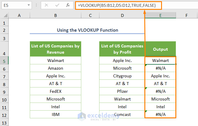
The above formula returns #N/A. The IFERROR function avoids that output.
=IFERROR(VLOOKUP(B5:B12,D5:D12,TRUE,FALSE),"")
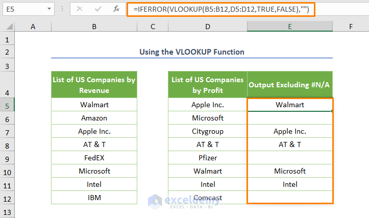
If you want to get the Duplicates or Unique as the output instead of getting the values duplicate values exactly, you may use the logical IF function.
=IF(ISERROR(VLOOKUP($B$5:B$12,$D$5:$D$12,TRUE,FALSE)),"Unique","Duplicates")
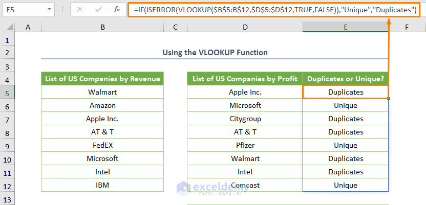
If you want to count duplicates, just use the COUNTIF function.
=COUNTIF(E5:E12,"Duplicates")
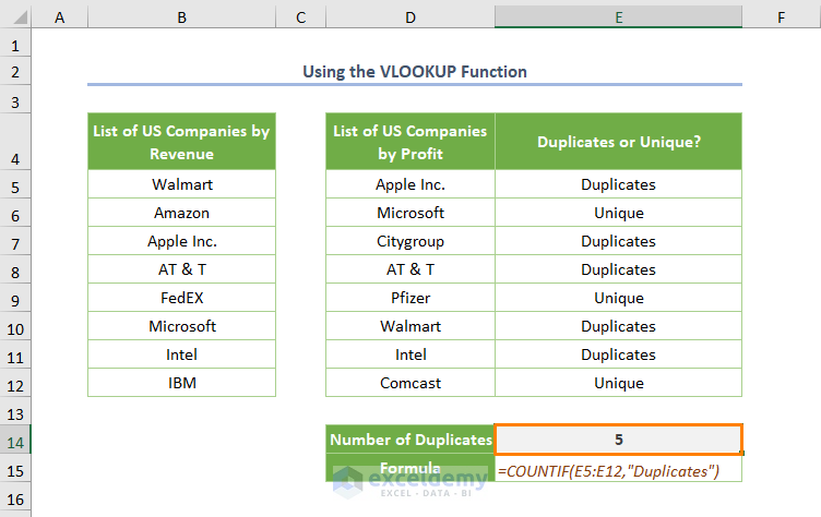
The cell E14 in the above picture shows the number of duplicates.
Read More: How to Count Duplicates Based on Multiple Criteria in Excel
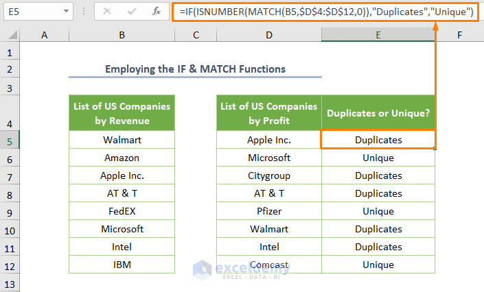
Method 6 – Using the IF and MATCH Functions to Count Duplicates in Excel
- Use this formula:
=IF(ISNUMBER(MATCH(B5,$D$4:$D$12,0)),"Duplicates","Unique")
B5 is the lookup value from List-1 and $D$4:$D$12 is the cell range for List-2.
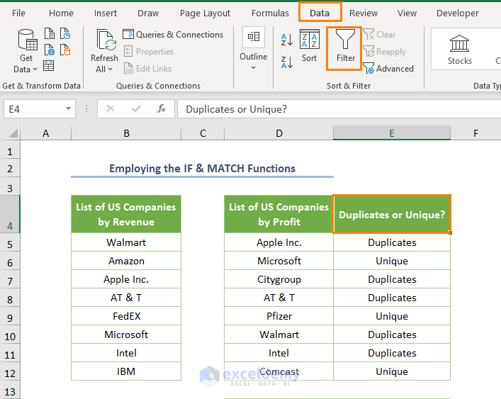
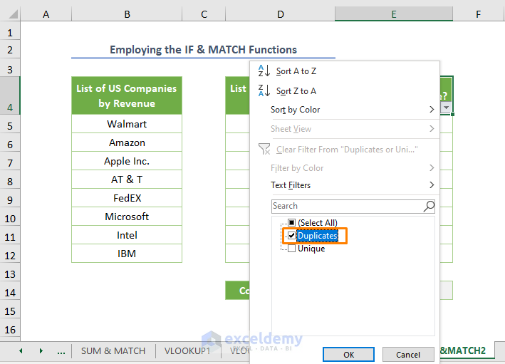
- Select E4.
- Click on the Filter option from the Sort & Filter ribbon in the Data tab.
- Click on the drop-down list and you’ll options.
- Check the box before Duplicates and uncheck the others.
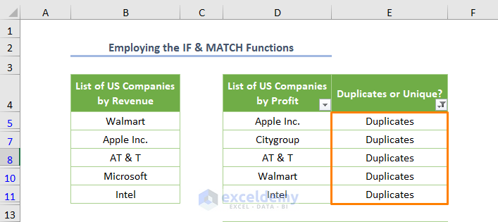
The output will be as follows.
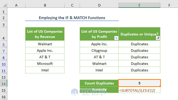
- Use the SUBTOTAL function to get the number of duplicates.
=SUBTOTAL(3,E5:E12)
3 refers to COUNTA that counts cells including the empty cells.
Read More: How to Count Occurrences Per Day in Excel
Method 7 – Counting Duplicates in Two Columns in Different Sheets
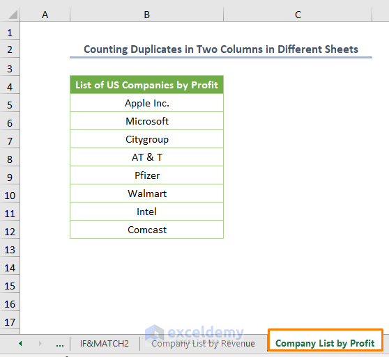
We want to count the number of duplicates along with two different sheets. The sheet Company List by Revenue contains the List-1.
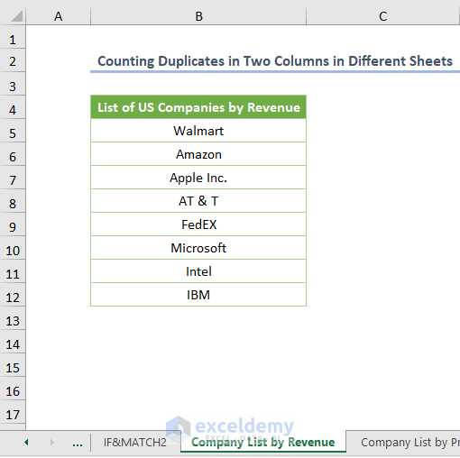
The second sheet Company List by Profit contains the List-2.
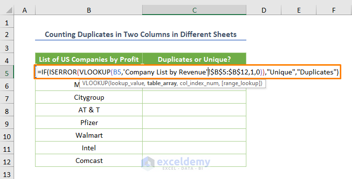
- Insert the following formula in the C5 cell of the second sheet.
=IF(ISERROR(VLOOKUP(B5,'Company List by Revenue'!$B$5:$B$12,1,0)),"Unique","Duplicates")
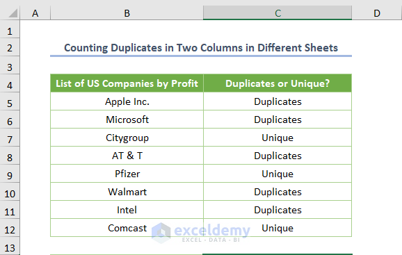
- Press Enter and use the Fill Handle Tool.
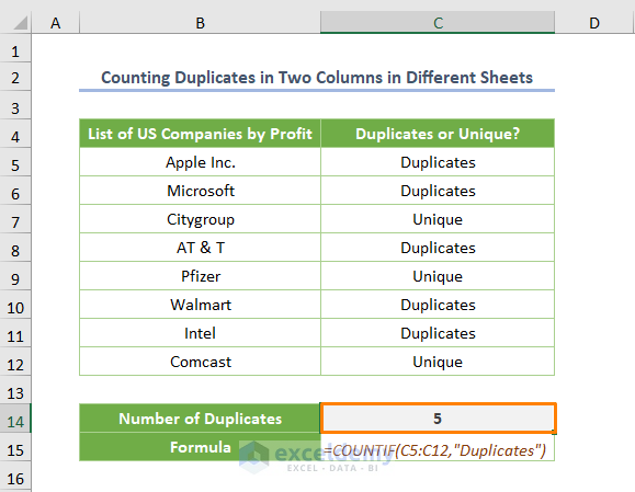
- If you want to count duplicates, use the following formula.
=COUNTIF(C5:C12,"Duplicates")
Method 8 – A Unique Method for Microsoft 365 Users to Count Duplicates
- Use the following formula:
=CHOOSE({1,2,3},UNIQUE(B5:C12),INDEX(UNIQUE(B5:C12),0,2), COUNTIFS(B5:C12,INDEX(UNIQUE(B5:C12),0,1),B5:C12,INDEX(UNIQUE(B5:C12),0,2)))
B5:C12 is the cell range of List-1 and List-2.
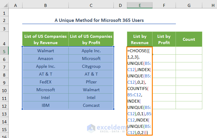
- If you press Enter, you’ll get the following output.
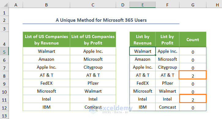
In the above picture, G8 and G11 return 2 because the value of their respective rows is duplicated.
The COUNTIFS function counts the number of duplicates for similar rows where the INDEX(UNIQUE(B5:C12),0,1) is the criterion for the first column that returns unique values. The INDEX(UNIQUE(B5:C12),0,2) is the criterion for the second column.
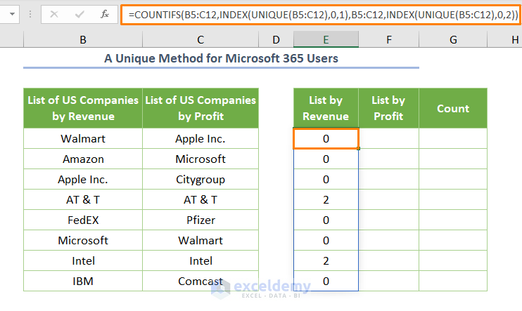
We used the CHOOSE function as the index_num 1,2,3 to get the value for getting the list of 3 arguments.
Things to Remember
- If you’re not a Microsoft 365 user, press CTRL + SHIFT + ENTER to apply an array function.
- You can put the dollar sign ($) as an absolute cell reference by pressing the F4 key while selecting a cell or range.
Download the Practice Workbook
<< Go Back to Count Duplicates in Excel | Learn Excel
Get FREE Advanced Excel Exercises with Solutions!


Thank You.
Hello Me,
You are most welcome. Your appreciation means a lot to us. You can explore more article related to these topic. Keep learning Excel with ExcelDemy.
Regards
ExcelDemy