The sample dataset showcases Salesman, Product, and Net Sales of a company. There is a blank cell and a number in Column B.
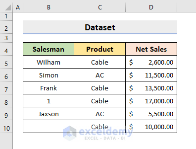
Method 1 – Using the Excel COUNTIFS Function to Count Filtered Cells with Text
STEPS:
- Select E5. Enter the formula:
=SUBTOTAL(103,B7)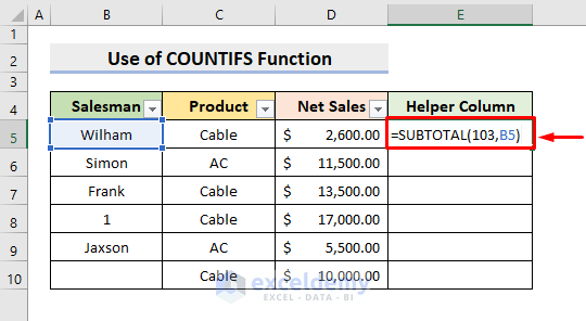
NOTE: 103, instead of 3, is used in the COUNTA function to exclude manually hidden rows. The COUNTA function returns 1 for a cell with a value, and 0 if empty.
- Press Enter and use the AutoFill tool to fill the series.
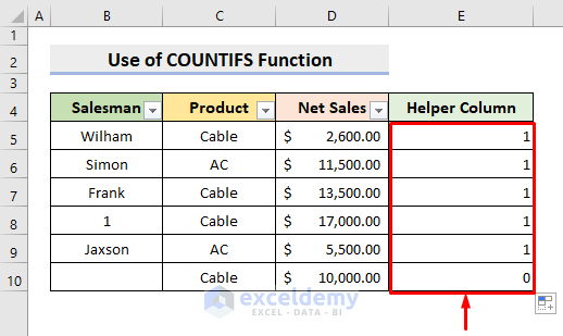
E10 is 0 as B10 is empty. With the Filter feature, the formula returns 0 for hidden rows whether blank or not.
- Select the drop-down symbol beside the header Product and select Cable.
- Click OK.
AC will be filtered and return Cable only.
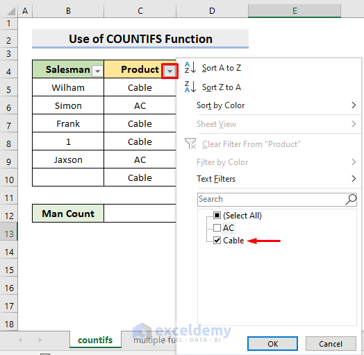
- Select C12 and enter the formula:
=COUNTIFS(B5:B10,"*",E5:E10,1)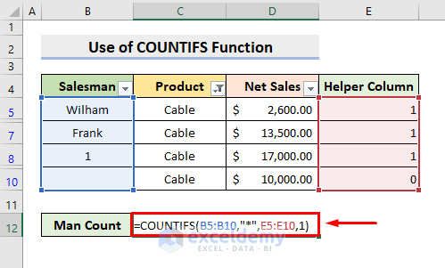
The first criteria is B5:B10, and the criterion Asterisk (*) matches the sequence of characters. The formula counts the text cells in the range. The second criteria is E5:E10 and the criterion is 1.
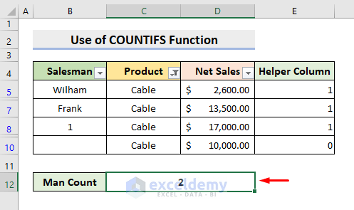
- Press Enter to see the count.
Method 2 – Combining the SUMPRODUCT, SUBTOTAL, INDIRECT, ROW & ISTEXT Functions to Count Filtered Cells with Text
STEPS:
- Select C12.

- Enter the formula:
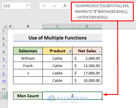
=SUMPRODUCT(SUBTOTAL(103, INDIRECT("B"&ROW(B5:B10))), --(ISTEXT(B5:B10)))- Press Enter to see the count.
Formula Breakdown
- ISTEXT(B5:B10)
checks for text values in each cell in B5:B10.
- ROW(B5:B10)
finds the row numbers in B5:B10.
- INDIRECT(“B”&ROW(B5:B10))
returns the individual references of all cells in the range.
- SUBTOTAL(103, INDIRECT(“B”&ROW(B5:B10)))
counts the cell references returned by the INDIRECT function and returns 1 for visible cells and 0 for hidden and empty cells.
- SUMPRODUCT(SUBTOTAL(103, INDIRECT(“B”&ROW(B5:B10))), –(ISTEXT(B5:B10)))
multiplies the elements in the same position of the arrays returned by the SUBTOTAL and ISTEXT functions and sums the final array.
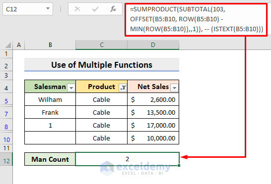
Method 3 – Combining the SUMPRODUCT, SUBTOTAL, OFFSET, MIN, ROW & ISTEXT Functions to Count Filtered Text Cells
STEPS:
- Select C12.
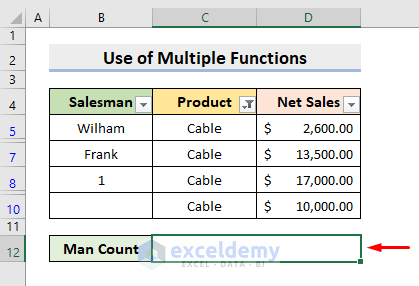
- Enter the formula:
=SUMPRODUCT(SUBTOTAL(103, INDIRECT("B"&ROW(B5:B10))), --(ISTEXT(B5:B10)))- Press Enter.
The count will be displayed.
Formula Breakdown
- ISTEXT(B5:B10)
checks text values in B5:B10.
- ROW(B5:B10)
returns the row numbers in B5:B10.
- MIN(ROW(B5:B10))
finds the smallest row number in B5:B10.
- OFFSET(B5:B10, ROW(B5:B10) – MIN(ROW(B5:B10)),,1)
return individual references of all cells in the range.
- SUBTOTAL(103, OFFSET(B5:B10, ROW(B5:B10) – MIN(ROW(B5:B10)),,1))
counts cell references and returns 1 for visible cells and 0 for hidden and empty cells.
- SUMPRODUCT(SUBTOTAL(103, OFFSET(B5:B10, ROW(B5:B10) – MIN(ROW(B5:B10)),,1)), — (ISTEXT(B5:B10)))
multiplies the elements in the same position of the arrays returned by the SUBTOTAL and ISTEXT functions and computes the sum of the final array.
Download Practice Workbook
Download the following workbook.
<< Go Back to With Text | Count Cells | Formula List | Learn Excel
Get FREE Advanced Excel Exercises with Solutions!

