How to Fix If Excel COUNT Function Not Working (4 Causes and Solutions)

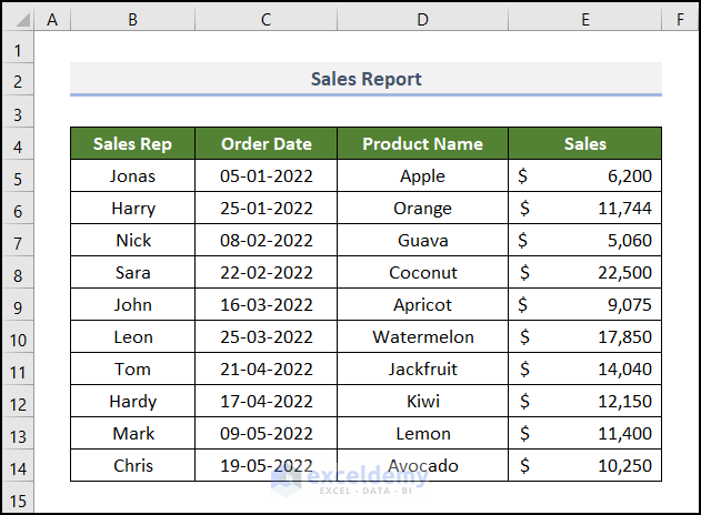
We will use a sales report for a particular grocery store. This dataset contains the Sales Rep, Order Date, Product Name, and their corresponding Sales amount in columns B, C, D, and E.

Read More: How to Use Different Types of COUNT Functions in Excel

Cause and Solution 1 – When Cells Containing COUNT Formula Are Formatted as Text

In this case, we count the Total Number of Sales reps in cell D16. To do this, we selected cell D16 and entered the following formula.

However, it doesn’t return the desired output. We can count the Sales Rep manually, and it’ll result in 10, but this number isn’t shown in the output cell.

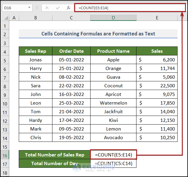
We’re having the same problem with cell D17. The reason behind this is the inappropriate formatting of these cells.

• Select cells in the D16:D17 range.

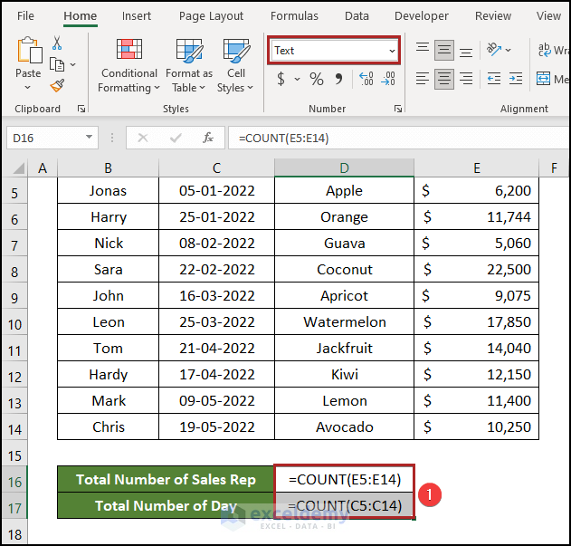
You can see that the cells are in Text format in the Number Format drop-down box in the Number group of commands. This is the reason the COUNT function is not working in Excel. So, let’s see the steps below to solve this problem.

Steps:

• Select cells in the D16:D17 range.
• Go to the Home tab.
• Click on the drop-down arrow in the Number Format box.
• From the drop-down list, choose General format.

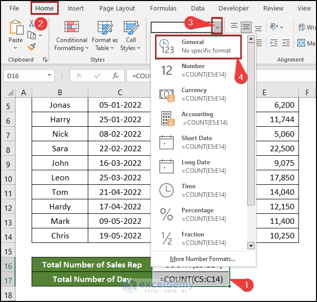
However, the outcome remains the same. The sheet remained unchanged.

To update the output,

• Go to cell D16.
• Double-click on the cell or press F2.
• Then, press ENTER.

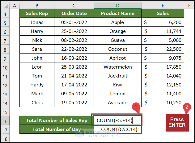
Now, we can see the updated and right output in cell D16.

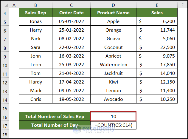
Similarly, update the result of cell D17. However, doing this is very time-consuming if there are many output cells. How can we overcome it?
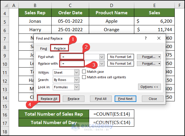
You can use the Find and Replace feature of Excel to deal with this phenomenon.

• Press CTRL+F to open the Find and Replace wizard.
• Move to the Replace tab.
• Enter the equal sign (=) in the Find what box.
• Enter another equal sign (=) in the Replace with box.
• Click on the Replace All button.

It’ll pop up with the message “All done. We made 2 replacements”.

You can see the two output cells, D16 and D17, exhibit the correct results.

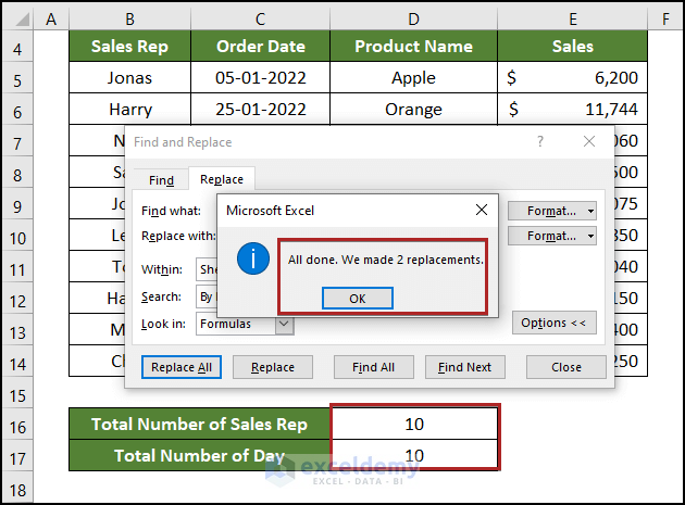
With this method, you can fix the outputs of various cells simultaneously, saving a lot of time and effort.

Read More: How to Count Numbers in a Cell in Excel

Cause and Solution 2 – If the Calculation Option Is Set as Manual

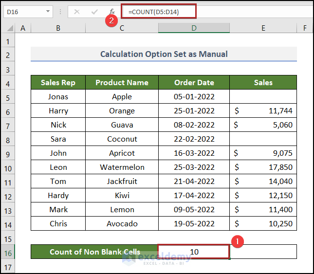
Here, we want to count the total number of days and the total number of Sales reps by counting the occurrence of the Sales amount.

• Select cell D16 and insert the formula below.

• Press the ENTER key.

• Bring the cursor to the right-bottom corner of cell D16 and it’ll look like a plus (+) sign. It’s the Fill Handle tool.
• Drag the tool to cell E16 to copy the formula in this cell.

However, it shows an erroneous result. We can count the cells manually in the Sales column. There are 8 cells with values, but our formula calculates them as 10.

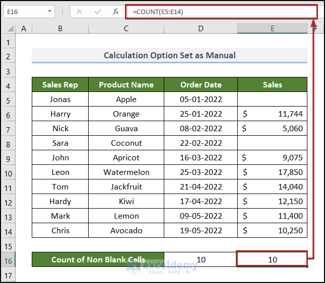
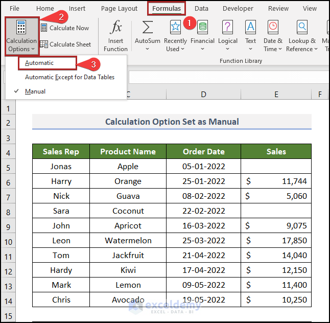
Why does it happen? The reason behind it is the action of the Calculation Option. Here, the Calculation Option is set as Manual. So, Fill Handle cannot work in this workbook now. So, we have to change it immediately to eliminate this error. Follow the simple steps below.

Steps:

• Go to the Formulas tab.
• Click on the Calculation Options drop-down on the Calculation group of commands.
• Select Automatic from the options.

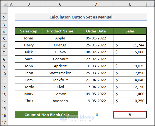
The output in cell E16 is changed to 8 from 10.

Read More: How to Find 5 Most Frequent Numbers in Excel

Cause and Solution 3 – When Cells Contain Text

Here, we tried to find the Total Number of Sales reps and the Total Number of Products in cells D16 and D17, respectively. Follow the image below to count the total Sales Reps.

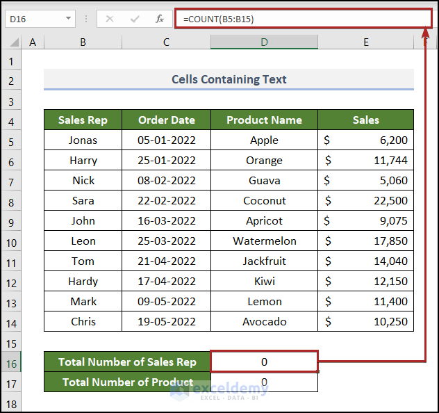
There are a total of 10 Sales Reps in this dataset. But the formula is returning 0 as an output in cell D16. Where’s the problem?
There’s no dilemma with our procedure. The main cause behind this matter is that the COUNT function ignores text values, and all the arguments are text values. So, follow our steps to make it correct.

Steps:

• Select cells in the B5:B14 range that we wanted to count.

Now, look at the Status Bar; you will find the total count of 10.

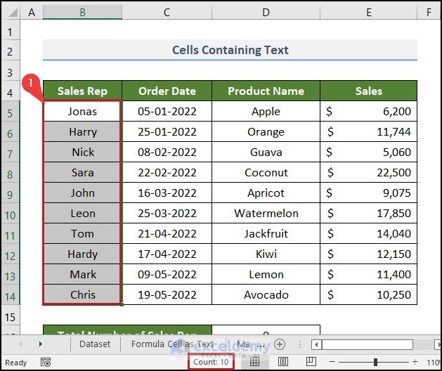
However, the best solution is to use the COUNTA function.

• Enter cell D16 and insert the following formula:

• Press ENTER.

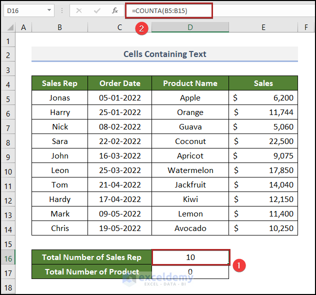
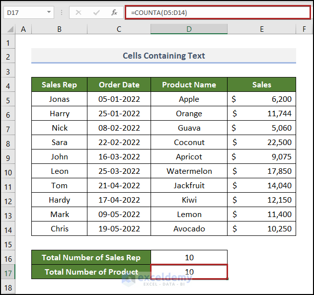
Do the same for the output of cell D17.

Cause and Solution 4 – When a Formula Returns Text Values

The COUNT function is also not compatible with the text output of other formulas. Here, we’ll discuss this topic. Let’s see it in action.
Using the IF function, we want to check which Order Date is after the Preferred Date and which is not. We’ll get a return of 1 and 0 for the TRUE value for FALSE.

• Select cell F5 and paste the formula below:

• Press ENTER.

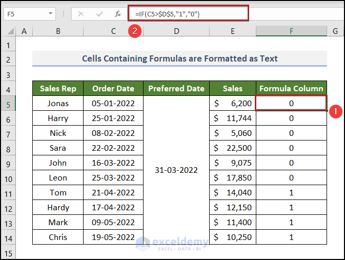
We’ll calculate the total number of days from the Formula Column. To do this, follow the below tasks.

• Select cell D16 and enter the following formula:

• Press ENTER.

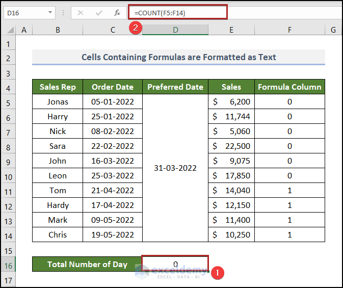
Here, the result is shown as 0. But the actual result should be 10. Why is it happening?
The main reason is the output in cells in the F5:F14 range. Notice the following image to understand it clearly.

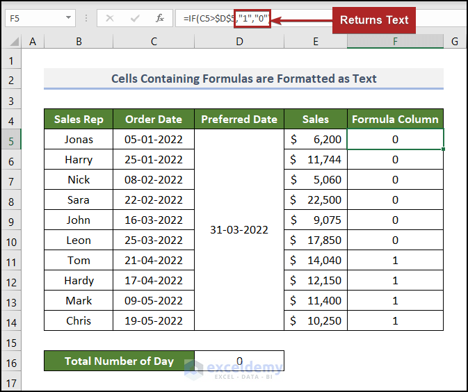
The above image shows double quotes around the digits 1 and 0 in the formula. So, the returned outputs are considered text values. The COUNT function would also work if the formula returns a number value. So, let’s see how we could fix this.

Steps:

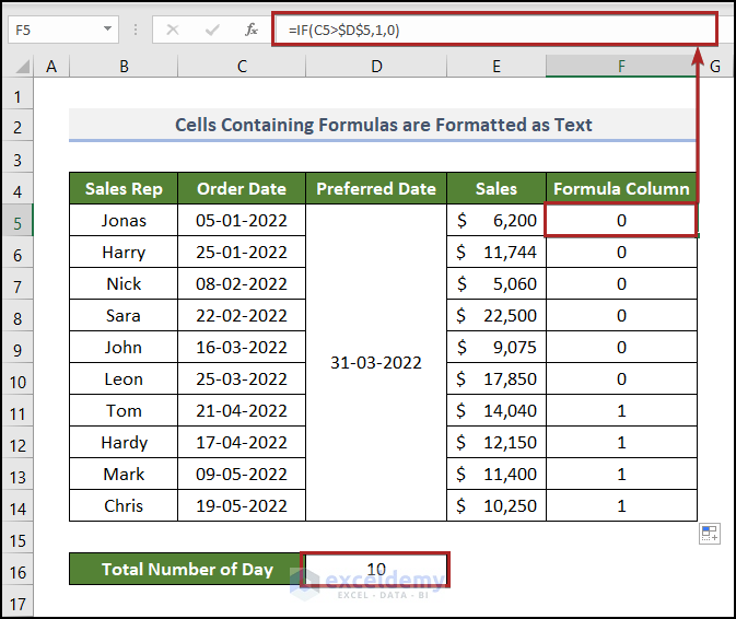
• Remove the double quotes from the formula of cell F5.

Now, the outputs in cells in the F5:F14 range are number values. The COUNT function also returns correct results as output in cell D16.

Download the Practice Workbook

Download the following Excel workbook to practice.