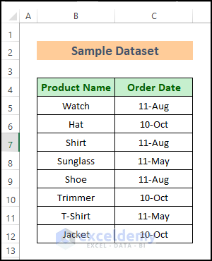
To demonstrate our methods, we’ll use the following dataset, containing columns for Product Name and Order Date. We used Excel 365 here, but the same methods should apply in other versions of Excel too.
Method 1 – Use COUNTIF Function
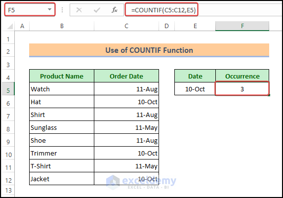
In our dataset, some dates are common to multiple products. Let’s use the COUNTIF function, which is used to count the number of cells that meet a criterion, to count the occurrences per day.
Steps:
- Activate Cell F6.
- Enter the following formula:
=COUNTIF(C5:C12,E6)- Press Enter button to return the result.
Read More: How to Count Duplicates in Column in Excel
Method 2 – Use SUMPRODUCT Function
The SUMPRODUCT function returns the sum of the products of corresponding ranges or arrays.
Steps:
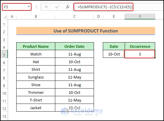
- Enter the following formula in Cell F6:
=SUMPRODUCT(--(C5:C12=E6))- Press Enter.
The occurrences for the day “10-Oct” are returned.
Breakdown of the Formula:
- (C5:C12=E6)
We check the value of Cell E6 against the array C5:C12 to see whether it matches or not. The result:
{FALSE;TRUE;FALSE;FALSE;FALSE;TRUE;FALSE;TRUE}
- –(C5:C12=E6)
The “—” sign before the formula will convert the previous result to binary format (0 for False and 1 for True). The result:
{0;1;0;0;0;1;0;1}
- SUMPRODUCT(–(C5:C12=E6))
The SUMPRODUCT function will sum the values. The result:
{3}
Read More: How to Count Duplicates in Two Columns in Excel
Method 3 – Use an Excel Pivot Table
Pivot Table is a tool that can calculate, summarize, and analyze data. It lets you see comparisons, patterns, and trends in the data.
Steps:
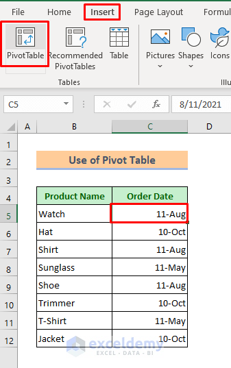
- Select any cell from the dataset.
- Click Insert > Pivot Table.
A Pivot Table dialog box will open up.
- Select Existing Worksheet.
- Select the cell from the Location bar where you want to create the Pivot Table. Here, we select cell E4.
- Click OK.
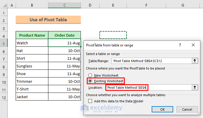
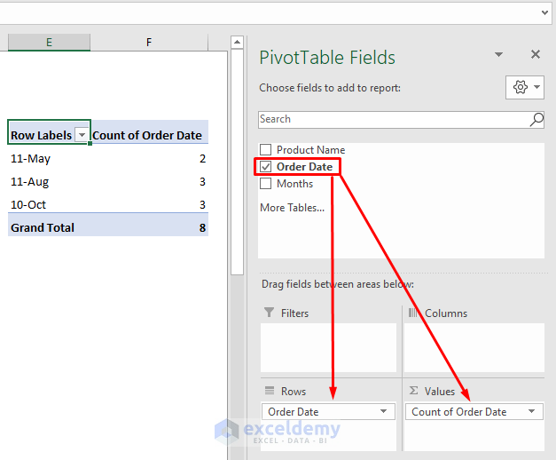
A “Pivot Table Field” box will appear on the right side of your sheet.
- Check only Order Date.
- Drag it to the Rows and Values fields.
The Pivot Table displays the occurrences for every unique day.
Read More: How to Count Duplicate Values in Multiple Columns in Excel
Method 4 – Use Excel VBA
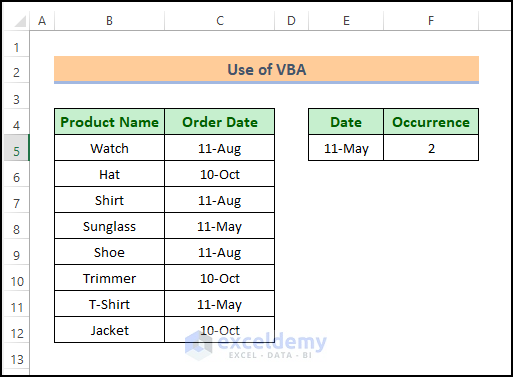
Let’s find the occurrences for the day “11-May” in Cell F6 using VBA code.
Steps:
- Right-click your mouse on the sheet name.
- Select the View Code option from the context menu.
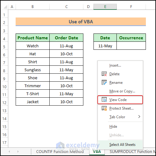
A VBA window will open up.
- Enter the following code:
Option Explicit
Sub Count_by_Day()
Dim ws As Worksheet
Dim output As Range
Dim dayvalue As String
Dim counter As Integer
Dim y As Integer
Set ws = Worksheets("Sheet")
Set output = ws.Range("F6")
dayvalue = ws.Range("E6")
counter = 0
For y = 5 To 12
If (ws.Range("C" & y)) = dayvalue Then
counter = counter + 1
End If
Next y
output = counter
End Sub- Press the Play button to run the codes.
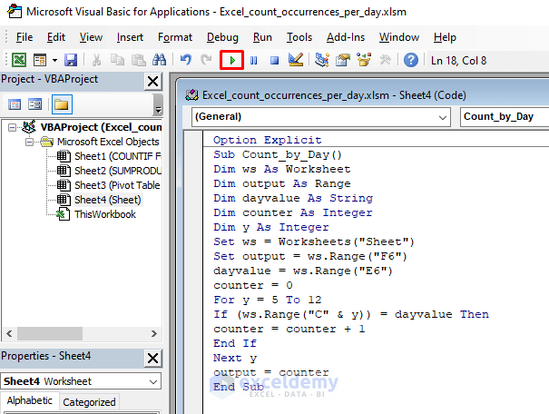
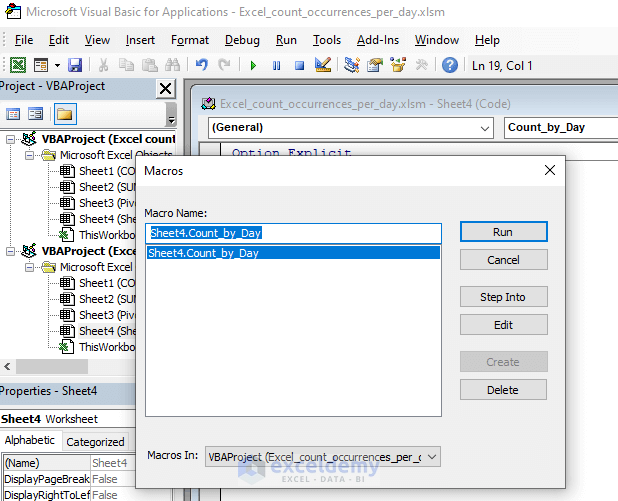
A dialog box named “Macro” will appear.
- Click Run.
The occurrences for that day are returned.
Read More: How to Count Duplicate Rows in Excel
Download Practice Workbook
Related Articles
- Count Number of Occurrences of Each Value in a Column in Excel
- Count the Order of Occurrence of Duplicates in Excel
- How to Count Duplicates Based on Multiple Criteria in Excel
<< Go Back to Count Duplicates in Excel | Learn Excel
Get FREE Advanced Excel Exercises with Solutions!

