How to Count Rows with a Formula in Excel (5 Methods)

Method 1 – Using the ROWS Function to Count Rows in Excel

Steps:

Enter the below formula in Cell D12:

=ROWS(B5:D10)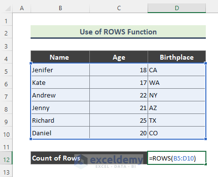

Here, the ROWS function returns the number of rows in the array: B5:D10.

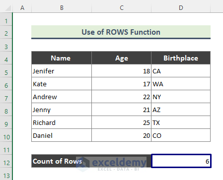
Press Enter.
You will get the number of rows that contain values.

Method 2 – Applying IF and COUNTA Functions to Count Rows

Steps:

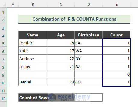
We will check whether rows in our dataset contain values or not. To do that, enter the following formula in Cell E5:

=IF(COUNTA(B5:D5)>0,1,0)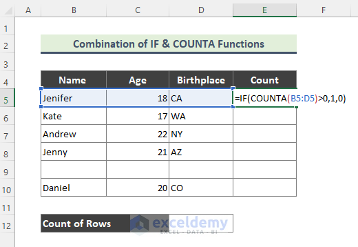

Here, the COUNTA function counts the number of non-empty cells in the range B5:D5. If the result of the COUNT formula is greater than 0, the IF function returns 1; otherwise, it returns 0.

Press Enter, and we will get the result below for Row 5.
Drag down the Fill Handle (+) to copy the formula to the rest of the cells.

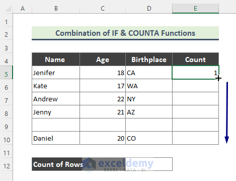
We get the following count for each of the rows.

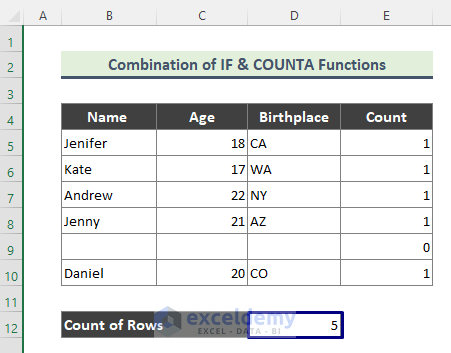
Use the SUM function, to get the total number of the rows having data.
Enter the following formula in Cell D12:

=SUM(E5:E10)

Press Enter.
Here is the total count of rows.

Method 3 – Inserting IF and COUNTBLANK Functions to Count Rows

Steps:

Enter the following formula in Cell E5:

=IF(COUNTBLANK(B5:D5)=3,0,1)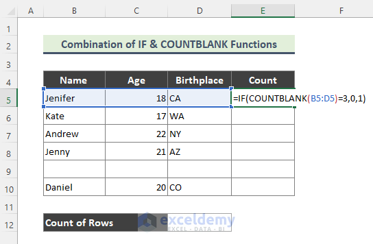

Here, the COUNTBLANK function counts the number of blank cells in the range B5:D5. In our dataset, we have three columns in each row. So, if all the cells are blank, the COUNTBLANK function will return 3. Later, the IF function will return 0 if the row is blank, otherwise 1.

Press Enter. We get the below result for each row.

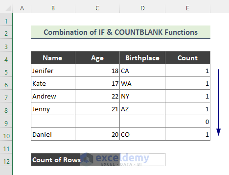
Similar to Method 2, we will sum up the above result to get the total non-empty row count of our dataset (B5:D10).
Enter the following formula in Cell D12:

=SUM(E5:E10)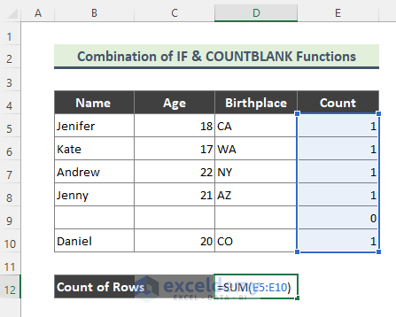

Press Enter.
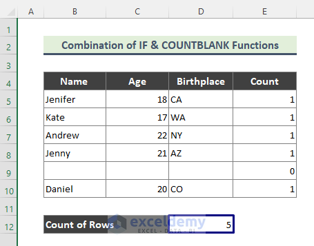
We found the total row count to be 5.

Method 4 – Using IF and COUNTIF Functions to Count Rows

Steps:

Enter the following formula in Cell E5:

=IF(COUNTIF(B5:D5,"")=3,0,1)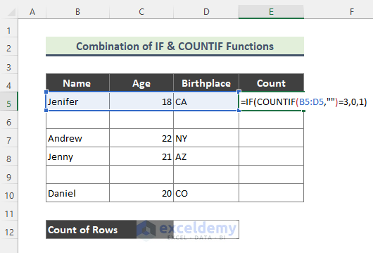

Here, the COUNTIF function counts the number of cells based on criteria. As we will need to find a blank cell in each row, the COUNTIF function counts blanks (“”) in the range B5:D5. When all three cells are blank in a row, the IF function returns 0, otherwise 1.

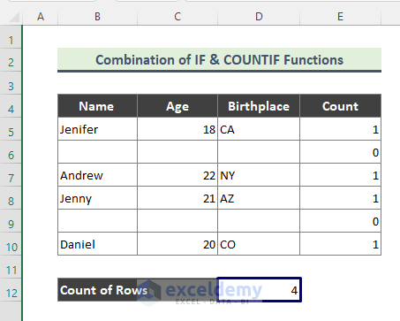
Press Enter to get the result below.

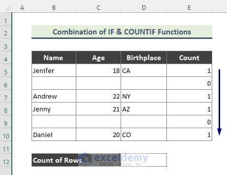
Add these individual counts of E5:E10 to get the total row count.
Enter the following formula in Cell D12:

=SUM(E5:E10)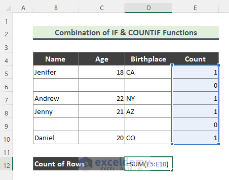

Press Enter.
We will get the following row count, 4.

Method 5 – Combining MMULT, TRANSPOSE, COLUMN, and SUM Functions to Count Rows

Steps:

Enter the following formula in Cell D12:

=SUM(--(MMULT(--(B5:D10=80),TRANSPOSE(COLUMN(B5:D10)))>0))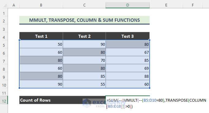

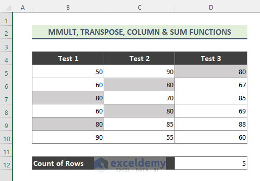
Press Enter.
We have found that 5 rows contain the value 80.

How does the Formula Work?

We are looking for the score ‘80’ in the dataset. The toughest part here is that the score ‘80’ can be present in any of the columns of the dataset and it can be in more than one column of the same row. So, the logical criteria used here are:

–(B5:D10=80): This logical criterion creates TRUE/FALSE results for each of the values in the range. Then, the double negative forces each TRUE/FALSE values to 1 and 0 and thus generate the below array:

{0,0,1;0,1,0;1,0,0;0,1,0;1,0,0;0,0,0}

TRANSPOSE(COLUMN(B5:D10)): Now, the COLUMN function is used to generate a numeric array of the right size. The COLUMN function returns the 3-column array {2,3,4}, and the TRANSPOSE function changes this array to the 3-row array {2;3;4}.
–(MMULT(–(B5:D10=80),TRANSPOSE(COLUMN(B5:D10)))>0): The MMULT function then runs and returns a 6 x 1 array result:

SUM(–({4;3;2;3;2;0}>0))

Now, we check for non-zero entries with > 0 and again force TRUE/FALSE to 1 and 0 with a double negative to get a final array inside the SUM function.

Finally, in the final array, 1 represents a row where the logical test returned TRUE. The summation returned by the SUM function is the count of rows (5) that contain the value 80.

Download the Practice Workbook

You can download the workbook to practice.

Count Rows with Formula.xlsx