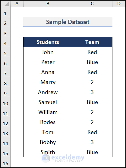
This is the sample dataset.
1. Using the Asterisk Sign with the COUNTIF Function Including Blank Cells
Steps:
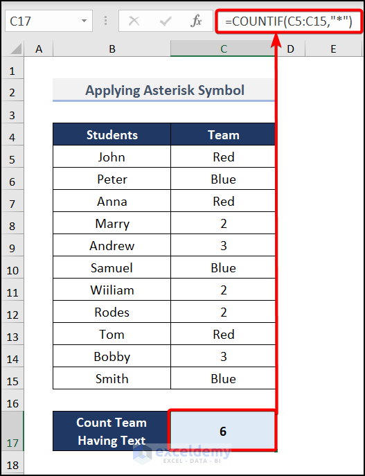
- Go to C17 and enter the formula:
The COUNTIF(C5:C15,”*”) syntax counts the cell containing text. The Asterisk symbol acts as text in the argument.
Read More: How to Use COUNTIF Function to Count Text from List in Excel
2. Using the Asterisk Sign with the COUNTIF Function Excluding Blank Cells
Steps:
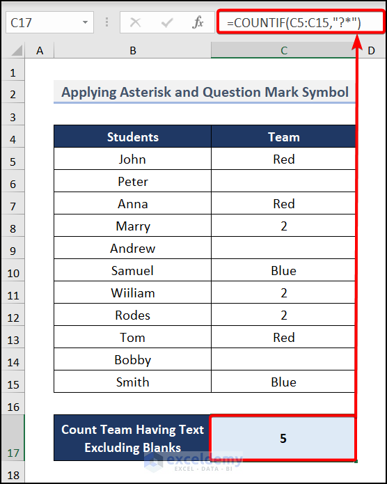
- Go to C17 and enter the formula:
The question mark excludes the blank cells and the Asterisk (*) is a text argument. Then the COUNTIF function counts the cells with text values excluding blanks.
Read More: [Fixed] COUNTIF Function with Wildcard Not Working in Excel
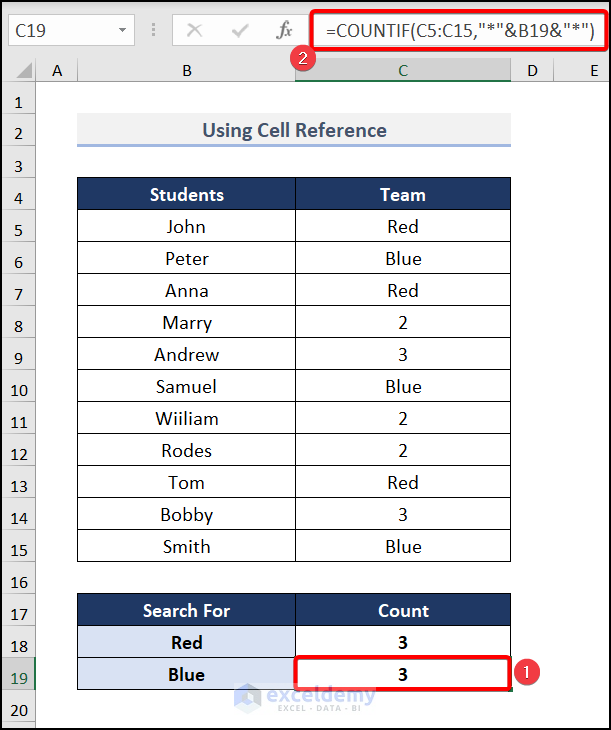
3. Counting Cells Using a Cell Reference.
Steps:
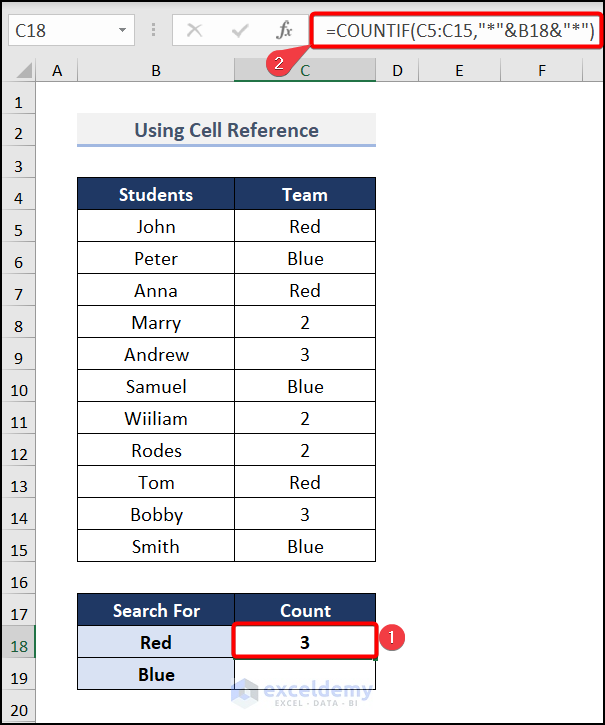
- Go to C18 and enter the formula:
Here,
B18 = Text that you want to search.
C5:C15= Entire data range.
COUNTIF(C5:C15,”*”&B18&”*”) takes the text value in B18 and counts it in C5:C15.
- Go to C19 and enter the formula:
The COUNTIF(C5:C15,”*”&B19&”*”) takes the text value in B19 and counts it in C5:C15.
This is the output.
Read More: Count Text at Start with COUNTIF & LEFT Functions in Excel
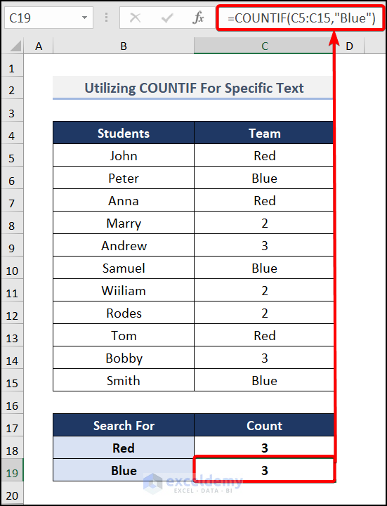
4. Utilizing the COUNTIF for a Specific Text
Steps:
- Go to C18 and enter the formula:
The COUNTIF counts the specific text “Red” in C5:C15.

- Go to C19 and enter the formula:
The COUNTIF counts the specific text “Blue” in C5:C15.
Using the COUNTIF Function to Count Cells That Contain Partial Text from Another Cell in Excel
Steps:
- Go to C17 and enter the formula:
The COUNTIF counts text starting with “R” in C5:C15.
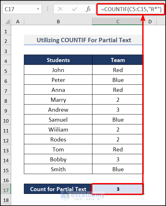
Note: The asterisk (*) after the partial text counts text starting with the alphabet. Before the partial text, it returns text that ends with the inserted argument.
Read More: [Solved!]: Excel COUNTIF Returning 0 Instead of Actual Value
Applying the COUNTIF Function to Count Cells That Contain Numbers from Another Cell in Excel
Steps:
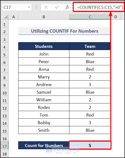
- Go to C17 and enter the formula:
The COUNTIF(C5:C15,”>0″) counts numbers greater than zero. It doesn’t count the blanks and negative values.
Utilizing the COUNTIF Function to Count Cells That Contain Text from a List
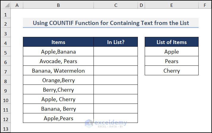
Steps:
- Go to C5 and enter the formula:
$E$5:$E$7 = The cells to be checked.
Formula Breakdown:
COUNTIF(B5,”*”&$E$5:$E$7&”*”)→ takes the text Apple, Pears, and Cherry as input and checks for a match in B5.
OR(COUNTIF(B5,”*”&$E$5:$E$7&”*”))→ The OR function returns the result of the COUNTIF function into the logical arguments. B5 has Apple on its list. Then, it will return 1 as it is considered a TRUE value. It returns 0 when text doesn’t match the item.
IF(OR(COUNTIF(B5,”*”&$E$5:$E$7&”*”)), “Yes”, “No”)→ The IF function shows the result Yes or No for the logical TRUE and FALSE. If the logical argument from the OR function shows 1, the IF function, considers it TRUE and returns Yes. 0 is shown for Boolean logic.
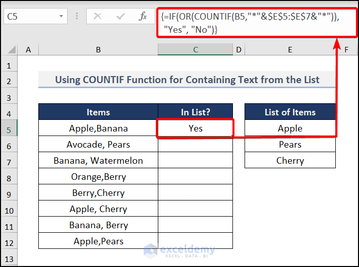
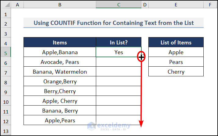
- Press ENTER and drag down the Fill Handle.
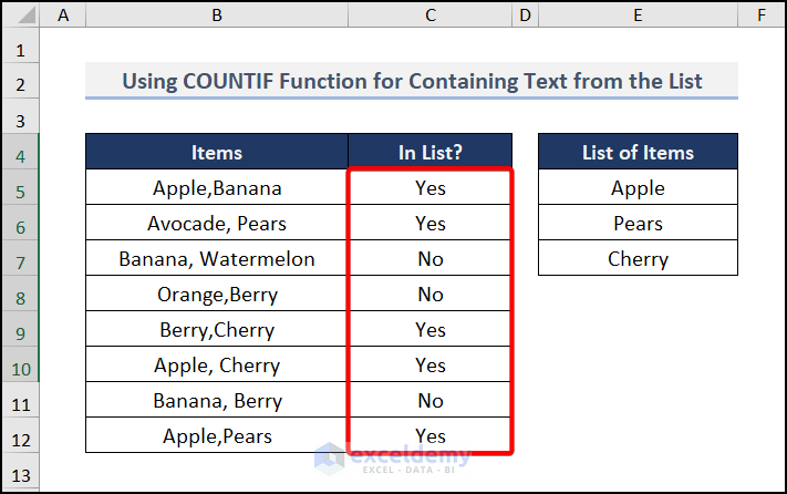
This is the output.
Read More: How to Use COUNTIF Function In Excel to Count Bold Cells
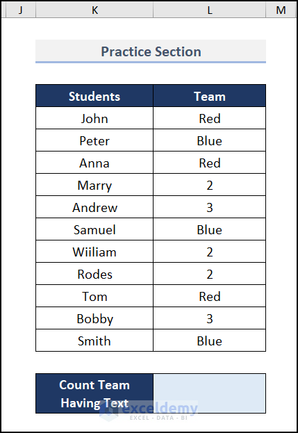
Practice Section
Practice here.
Download Practice Workbook
Download the following practice workbook.
<< Go Back to Excel COUNTIF Function | Excel Functions | Learn Excel
Get FREE Advanced Excel Exercises with Solutions!

