The COUNTIF Function
The COUNTIF function counts the number of data that matches a criterion. You can calculate both text values and numeric values.
Syntax:
=COUNTIF(range, criteria)Arguments:
range: range of cells to match the criteria.
criteria: the logic that determines the cells to be counted.
Example 1 – Apply the COUNTIF and the COUNTA Functions to Find the Percentage of a Specific Value in Excel
- Select G5 and enter the formula below:
=COUNTIF($D$5:$D$12,F5)/COUNTA($D$5:$D$12)- Press Enter.
- Select Number Format in the Home tab.
- Change the cell format to Percentage.
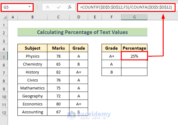
- Use the Fill Handle to copy the formula to the cells below.
This is the output.
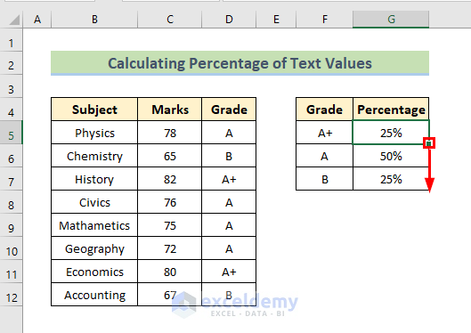
Read More: COUNTIF Between Two Cell Values in Excel
Example 2 – Calculate the Percentage of Numeric Values Using the COUNTIF and the COUNTA Functions in Excel
- Select F5 and enter the formula below:
=COUNTIF(C5:$C$12,">=80")/COUNTA(C5:$C$12)- Press Enter.
- Select Number Format in the Home tab.
- Change the cell format to Percentage.
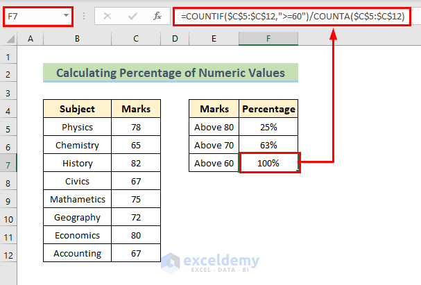
You will see the result in percentage (marks above 80).
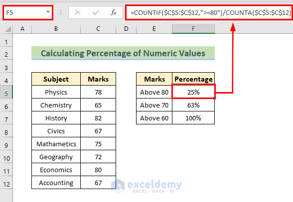
- Calculate the percentage of marks above 70 in F6:
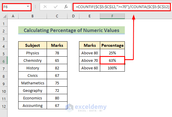
- Calculate the percentage of marks above 60 in F7:
Read More: How to Calculate Frequency Using COUNTIF Function in Excel
How to Determine the Percentage Range in Excel
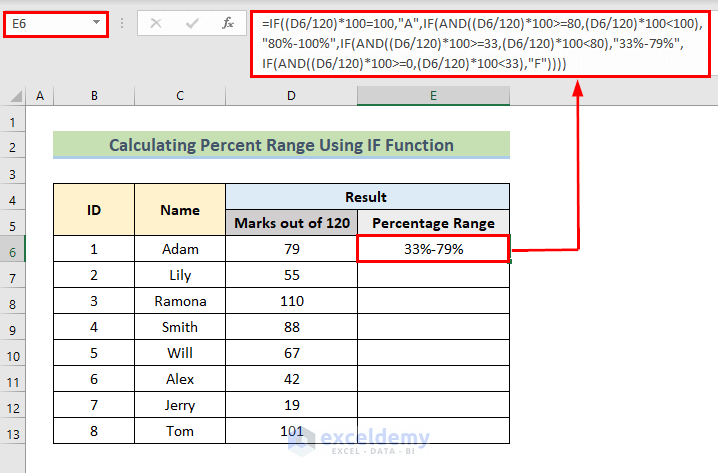
- Select E6 and enter the formula below:
=IF((D6/120)*100=100,"A",IF(AND((D6/120)*100>=80,(D6/120)*100<100),"80%-100%",IF(AND((D6/120)*100>=33,(D6/120)*100<80),"33%-79%",IF(AND((D6/120)*100>=0,(D6/120)*100<33),"F"))))- Press Enter.
This is the output.
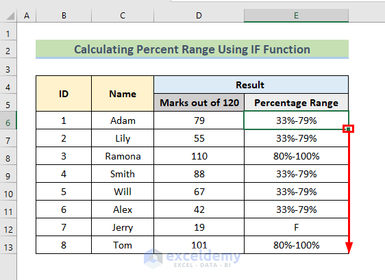
- Drag down the Fill Handle to see the result in the rest of the cells.
This is the final output.
In the formula:
The first logical test checks if (D6/120)*100 is equal to 100. If true, it returns 100%; if false, it moves to the second logical test.
The second logical test checks if (D6/120)*100>=80,(D6/120)*100<100. If true, it returns 80%-99%; if false, it moves to the third logical test.
The third logical test checks if (D6/120)*100>=33,(D6/120)*100<80. If true, it returns 33%-80%; if false, it moves to the fourth and final logical test.
The formula checks if (D6/120)*100>=0,(D6/120)*100<33). If true, it returns F.
Read More: How to Use COUNTIF Function with Array Criteria in Excel
How to Use the COUNTIFS Function to Calculate Percentage in Excel
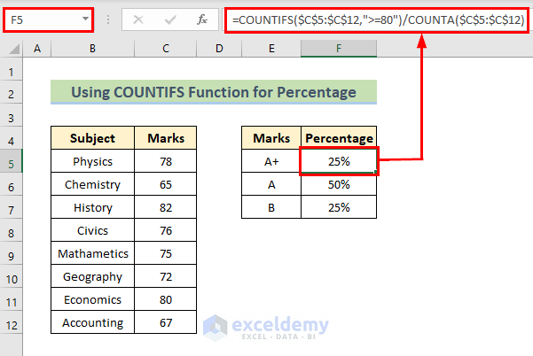
- Select F5 and enter the following formula:
=COUNTIFS($C$5:$C$12,">=80")/COUNTA($C$5:$C$12)
[/wpsm_box]
- Press Enter.
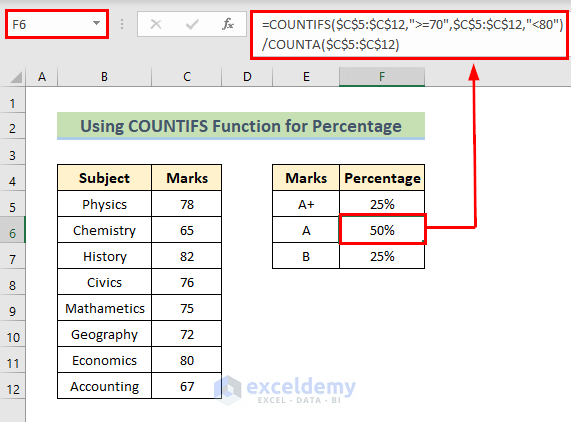
- Enter the following formula in CF6.
=COUNTIFS($C$5:$C$12,">=70",$C$5:$C$12,"<80")/COUNTA($C$5:$C$12)- Press Enter.
- Select F7 and use the following formula.
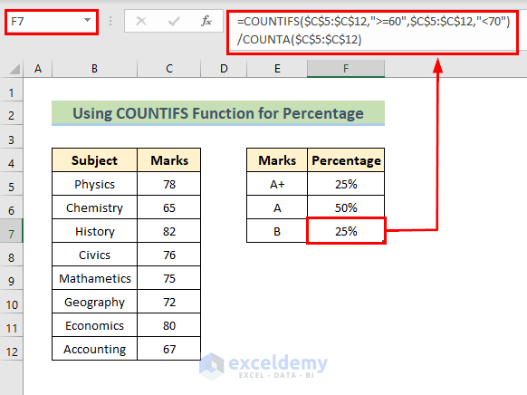
=COUNTIFS($C$5:$C$12,">=60",$C$5:$C$12,"<70")/COUNTA($C$5:$C$12)- Press Enter.
This is the output.
Read More: Excel COUNTIF to Count Cells Greater Than 1
Download Practice Workbook
Download the practice workbook.
Related Articles
- How to Use COUNTIF for Non Contiguous Range in Excel
- COUNTIF Function to Count Cells That Are Not Equal to Zero
- How to Use COUNTIF Function in Excel Greater Than Percentage
- How to Compare Two Columns Using COUNTIF Function
- How to Use Excel COUNTIF Between Time Range
<< Go Back to Excel COUNTIF Function | Excel Functions | Learn Excel
Get FREE Advanced Excel Exercises with Solutions!


Help – not sure where I’m going wrong. I’m trying to calculate the participation % among 21 members of our board. I have the board members going across the top row, the months going down the first column, and I’ve entered the letter “X” for each member that attended.
Initially, I used this formula: =COUNTIF(B2:V2, “X”)/COUNTA(B2:V2) but the result was 100%, so then I used this formula based on the instructions above: =COUNTIF(B2:V2, A1)/COUNTA($B$2:$V$2), but I get the same result.
The match comes out to 85.7%, but I can’t see where I’m going wrong. Any help is appreciated!
Hello jean,
Thank you for sharing your problem with us!
In order to calculate the participation percentage, you can follow the instructions below.
1. Simply choose a blank cell.
2. Insert the following formula:
=COUNTIF($C$5:$C$25, E5)/COUNTA($C$5:$C$25)Thus you can calculate the participation percentage.
Note:
1. The formula you used did not work because you did not lock the cell range using absolute reference.
2. Another reason is don’t leave the cells blank for the choosen cell range.