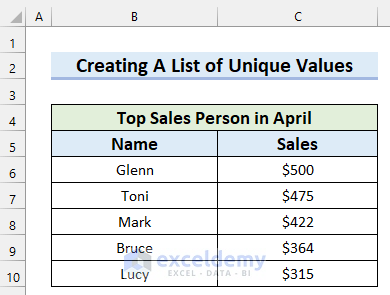
To demonstrate the different methods to obtain unique values from columns in multiple sheets, we will use 3 Excel sheets as a dataset. Each of them contains the Top Sales Person list for a month. The first sheet contains the Top Sales Person in April list.
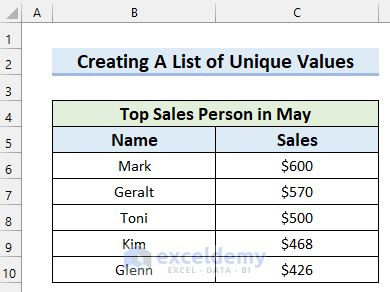
The second sheet contains the Top Sales Person in May list.
And the third sheet contains the Top Sales Person in June list.
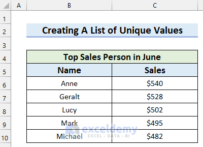
These sheets have repeating values in them. Let’s create a list of unique values from these 3 sheets.
Method 1 – Creating a List of Unique Values from Multiple Sheets Manually by Using Sort & Filter Group
Steps:
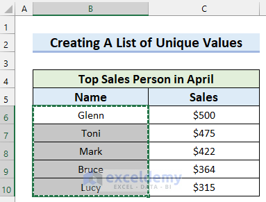
- Select the data from the first sheet.
- Press CTRL+C to copy the selected values.
- Go to the sheet where you want to create the unique value list.
- Select the cell from where you want the list to begin. Here, cell B5.
- Press CTRL+V to paste the values you copied.
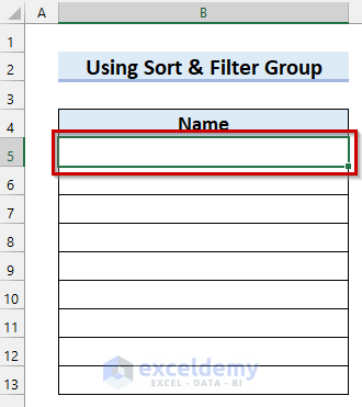
The values from the first sheet are returned.
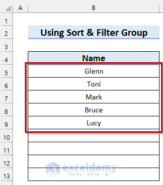
- In the same way, copy the values from the other sheets too.
We now have all the values from the 3 sheets in column B.
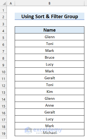
We can now create a list of unique values from this list.
- Go to the Data tab.
- Select Advanced.
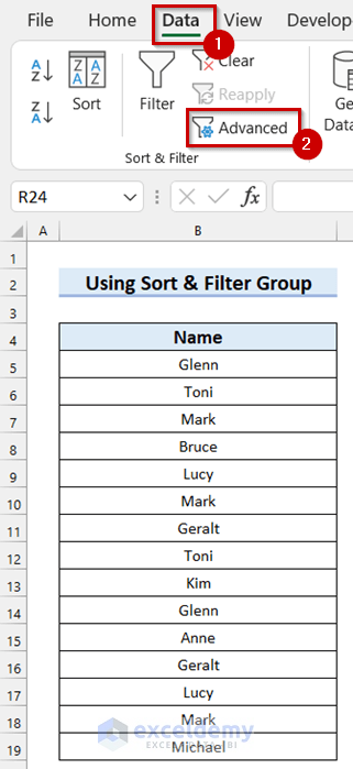
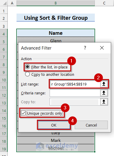
A dialog box names Advanced Filter will open.
- Select Filter the list, in-place.
- Select the List range.
- Check the Unique records only option.
- Click OK.
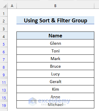
The list of unique values from multiple sheets is returned.
Method 2 – Using Power Query to Create List of Unique Values from Multiple Sheets in Excel
Steps:
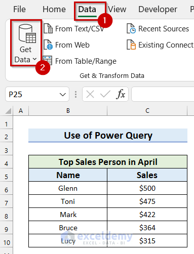
- Go to the Data tab.
- Select Get Data.
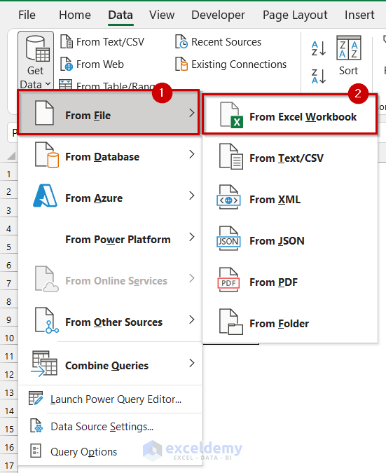
A drop-down menu appears.
- Select From File.
- Select From Excel Workbook.
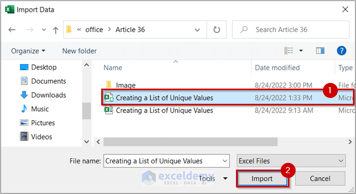
A file dialog box will open.
- Select the file from where you want to import the data.
- Select Import.
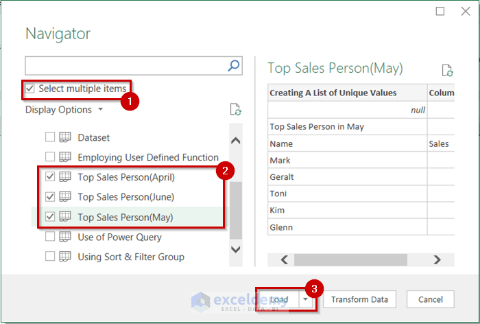
The Navigator will open.
- Check Select multiple items.
- Select the sheets from which you want to create your list of unique values.
- Select Load.
The Power Query Editor opens and our sheets are inserted as tables. As in the following picture, we don’t need the first two rows of the table.
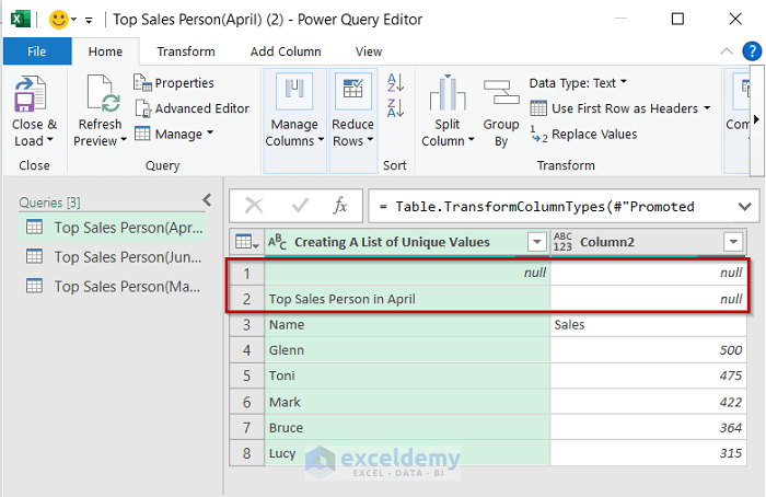
To delete the first two rows from the table:
- Select Reduce Rows.
- Select Remove Rows.
- Select Remove Top Rows.

A dialog box will appear.
- Select the number of rows you want to remove. Here 2, as we want to remove the first two rows.
- Click OK.

The first 2 rows are removed from the table.
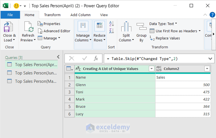
- Remove the first two rows from the second table by following the previous steps.
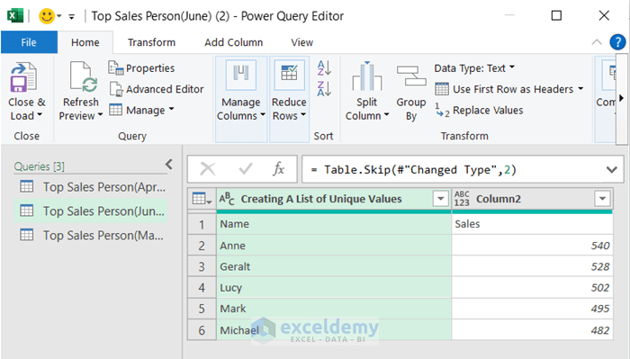
- Remove the first two rows from the third table by following the previous steps.
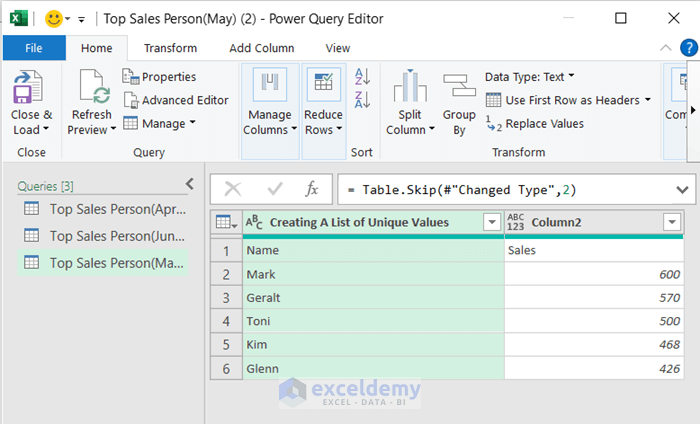
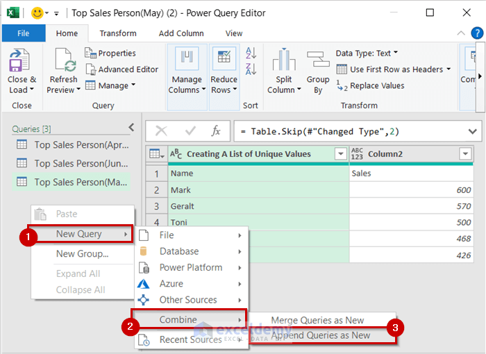
- Right-click anywhere in the Queries section.
- Select New Query.
- Select Combine.
- Select Append Queries as New.
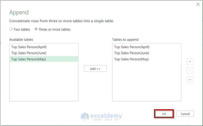
A dialog box named Append will appear.
- Select Three or more tables.
- Select the table you want to add.
- Select Add.
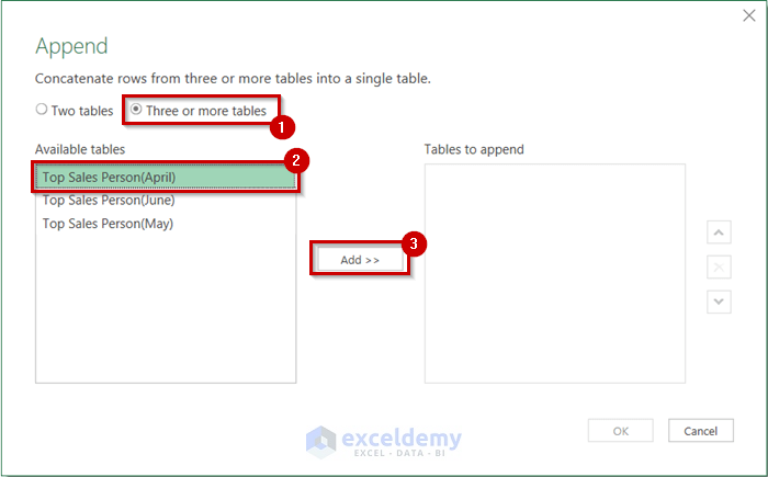
The selected table is added to Tables to append.

- In the same way, add the other tables.
- Click OK.
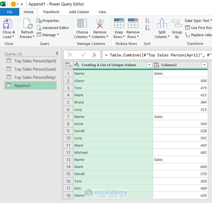
The values from the 3 tables are combined into one.
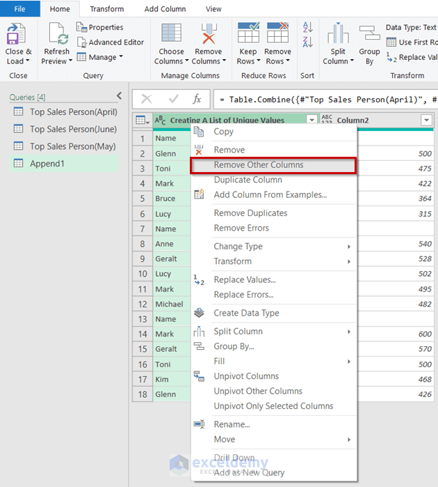
We only need the first column, so we remove the other columns:
- Select the column.
- Right-click on the column.
- Select Remove Other Columns.
The other columns are removed from the table.
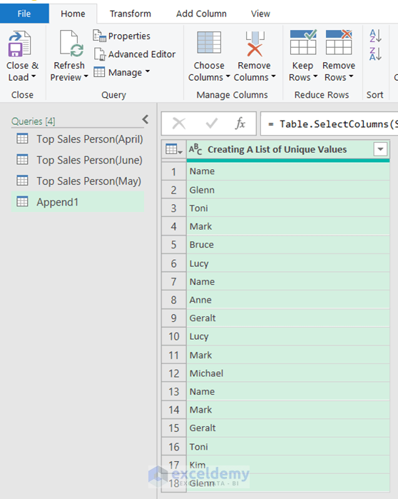
Now we can remove the duplicate values to get the list of unique values.
- Select the column.
- Right-click on the column.
- Select Remove Duplicates.
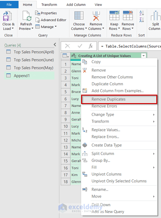
What remains is a list of unique values.
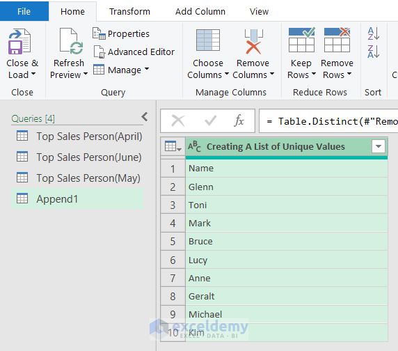
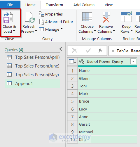
For clarity, I have changed the header of my table.
- Select Close & Load.
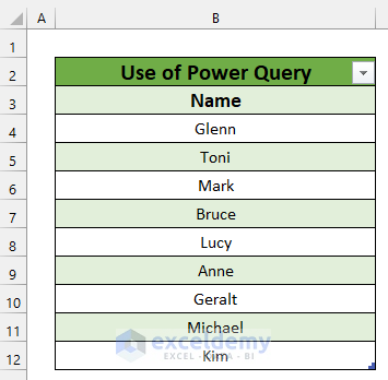
The list of unique values looks like this:
Method 3 – Using a User-Defined Function to Create List of Unique Values from Multiple Sheets
Steps:
First we need to create a user-defined function using VBA code.
- Go to the Developer tab.
- Select Visual Basic.
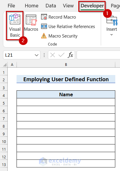
The Visual Basic window will open.
- Go to the Insert tab.
- Select Module.
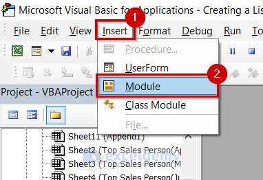
A Module window will open.
- In that Module enter the following code.
Function split_function(split_text As String, Optional delimiter As String = ",") As Variant
split_function = Split(split_text, delimiter)
End Function
Code Breakdown
- We create a Function named split_function as Variant.
- We declare split_text as String and an Optional argument delimiter as string, setting it as “,”.
- We use the Split function with split_text as expression and delimiter. The function will return a one-dimensional array.
- We end the Function.
- Save the code and go back to your worksheet.
- Select the cell where you want your list of unique values to begin. Here, cell B5.
- In cell B5 enter the following formula:
=UNIQUE(TRANSPOSE(split_function(TEXTJOIN(",",,'Top Sales Person(April):Top Sales Person(June)'!B6:B10))))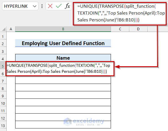
Formula Breakdown
- TEXTJOIN(“,”,,’Top Sales Person(April):Top Sales Person(June)’!B6:B10) —-> the TEXTJOIN function will join the texts in range B6:B10 from sheet range ‘Top Sales Person(April):Top Sales Person(June)’! with a delimiter “,”.
- Output: “Glenn,Toni,Mark,Bruce,Lucy,Mark,Geralt,Toni,Kim,Glenn,Anne,Geralt,Lucy,Mark,Michael”
- split_function(TEXTJOIN(“,”,,’Top Sales Person(April):Top Sales Person(June)’!B6:B10)) —-> turns into
- split_function(“Glenn,Toni,Mark,Bruce,Lucy,Mark,Geralt,Toni,Kim,Glenn,Anne,Geralt,Lucy,Mark,Michael” ) —-> the split_function will return a one-dimensional array containing specific numbers or substring after each delimiter.
- Output: {“Glenn”,”Toni”,”Mark”,”Bruce”,”Lucy”,”Mark”,”Geralt”,”Toni”,”Kim”,”Glenn”,”Anne”,”Geralt”,”Lucy”,”Mark”,”Michael”}
- split_function(“Glenn,Toni,Mark,Bruce,Lucy,Mark,Geralt,Toni,Kim,Glenn,Anne,Geralt,Lucy,Mark,Michael” ) —-> the split_function will return a one-dimensional array containing specific numbers or substring after each delimiter.
- TRANSPOSE(split_function(TEXTJOIN(“,”,,’Top Sales Person(April):Top Sales Person(June)’!B6:B10))) —-> turns into
- TRANSPOSE({“Glenn”,”Toni”,”Mark”,”Bruce”,”Lucy”,”Mark”,”Geralt”,”Toni”,”Kim”,”Glenn”,”Anne”,”Geralt”,”Lucy”,”Mark”,”Michael”}) —-> the TRANSPOSE function will convert the the horizontal array to a vertical array.
- Output: {“Glenn”;”Toni”;”Mark”;”Bruce”;”Lucy”;”Mark”;”Geralt”;”Toni”;”Kim”;”Glenn”;”Anne”;”Geralt”;”Lucy”;”Mark”;”Michael”}
- TRANSPOSE({“Glenn”,”Toni”,”Mark”,”Bruce”,”Lucy”,”Mark”,”Geralt”,”Toni”,”Kim”,”Glenn”,”Anne”,”Geralt”,”Lucy”,”Mark”,”Michael”}) —-> the TRANSPOSE function will convert the the horizontal array to a vertical array.
- UNIQUE(TRANSPOSE(split_function(TEXTJOIN(“,”,,’Top Sales Person(April):Top Sales Person(June)’!B6:B10)))) —-> turns into
- UNIQUE({“Glenn”;”Toni”;”Mark”;”Bruce”;”Lucy”;”Mark”;”Geralt”;”Toni”;”Kim”;”Glenn”;”Anne”;”Geralt”;”Lucy”;”Mark”;”Michael”}) —-> the UNIQUE function will return a list of distinct values.
- Output: {“Glenn”;”Toni”;”Mark”;”Bruce”;”Lucy”;”Geralt”;”Kim”;”Anne”;”Michael”}
- UNIQUE({“Glenn”;”Toni”;”Mark”;”Bruce”;”Lucy”;”Mark”;”Geralt”;”Toni”;”Kim”;”Glenn”;”Anne”;”Geralt”;”Lucy”;”Mark”;”Michael”}) —-> the UNIQUE function will return a list of distinct values.
- Press ENTER to return our unique values list.
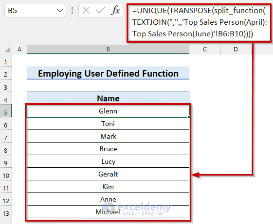
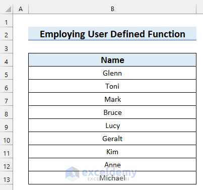
Here is the final list of unique values from multiple sheets in Excel.
Method 4 – Using VBA to Create a List of Unique Values from Multiple Sheets in Excel
Steps:
- Go to the Developer tab.
- Select Visual Basic.
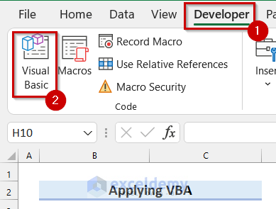
The Visual Basic window will open.
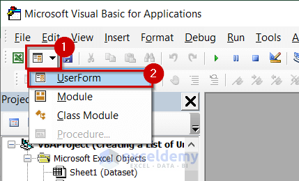
- Select the drop-down option from UserForm.
- Select UserForm.
- The UserForm will appear.
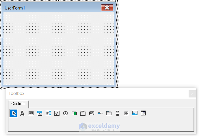
- Click on the Label from Toolbox.
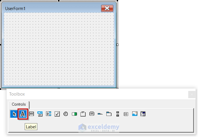
- Click and drag your mouse cursor where you want the label of your UserForm.
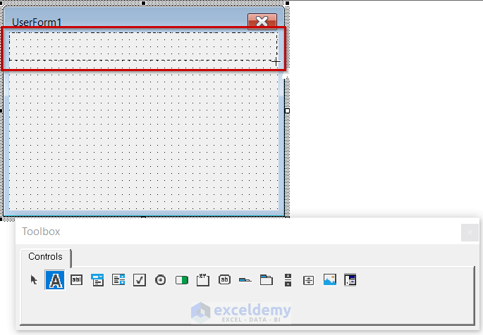
The Label is created.
- Right-click on the Label.
- Select Properties.
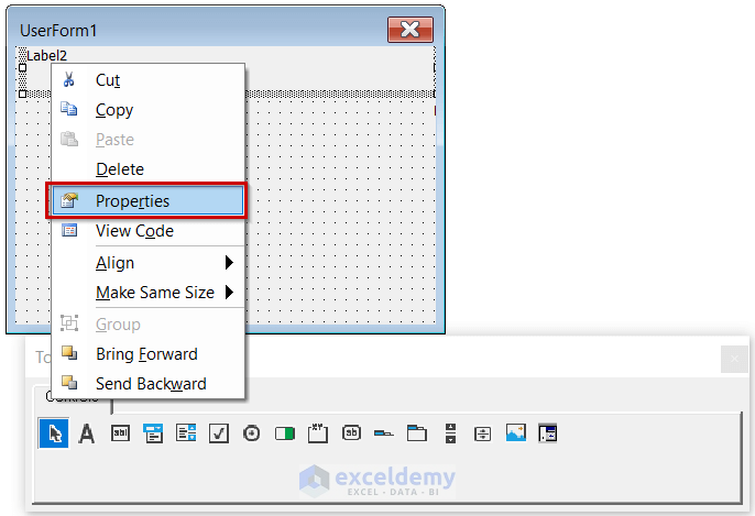
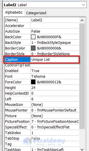
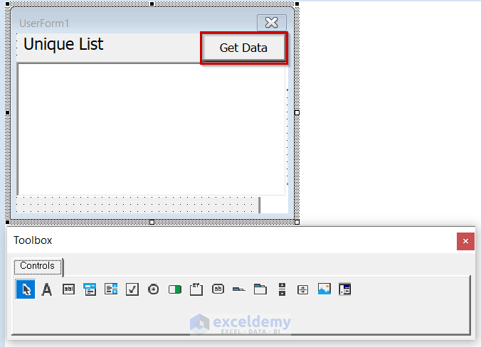
- Change the Caption if you want. Here, I changed mine to Unique List.
- Select CommandButton from the toolbox.
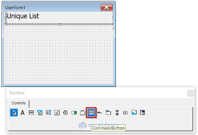
- Click and drag the mouse cursor where you want the CommandButton.
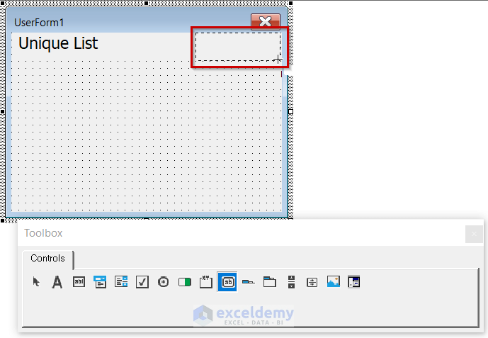
The CommandButton is inserted in the UserForm.

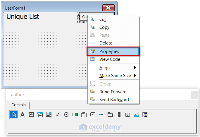
- Right-click on the CommandButton.
- Select Properties.
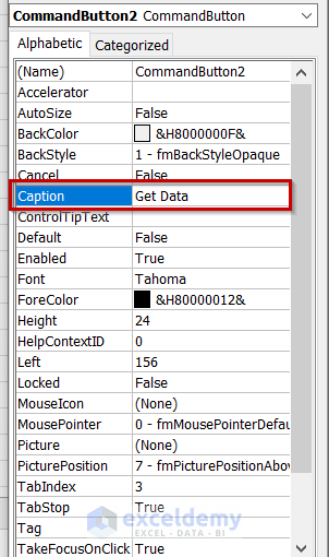
- Change the properties if you want. Here, I changed my caption to Get Data.
- Select ListBox.
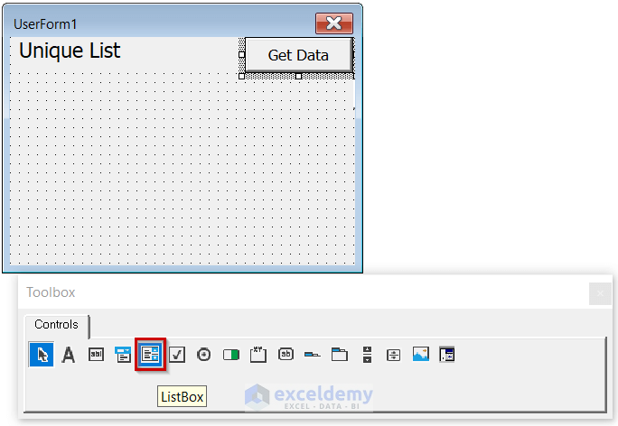
- Click and drag your mouse cursor where you want the ListBox.
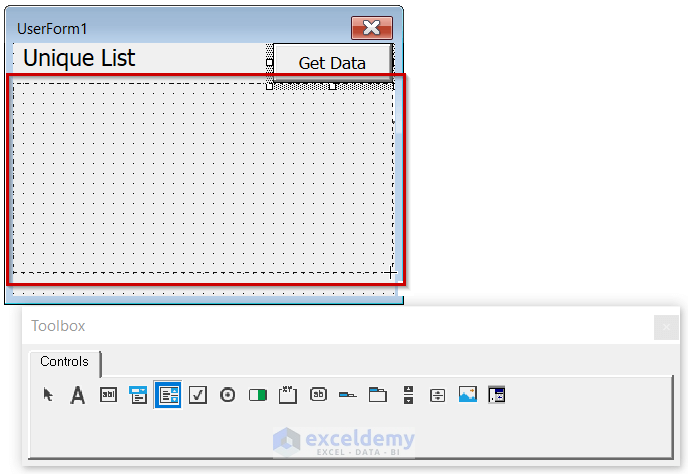
The list box is inserted into the UserForm.
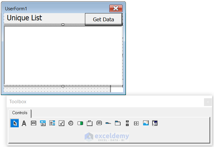
- Double-click anywhere in the marked part.
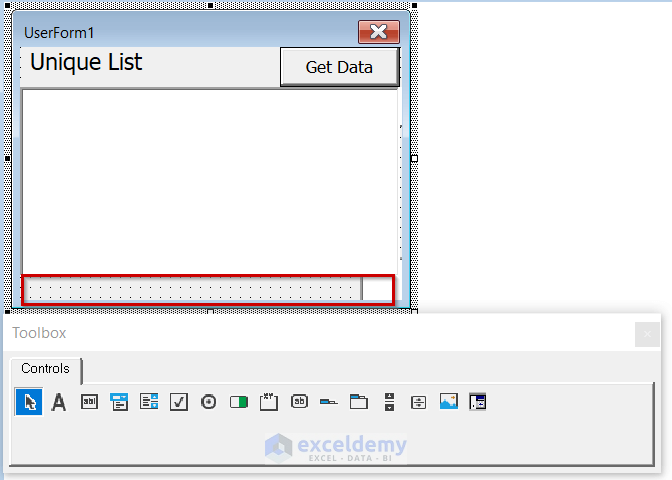
A Module will open with a Private Sub Procedure named UserForm_Click().
- Select the marked drop-down option.
- Select Initialize.
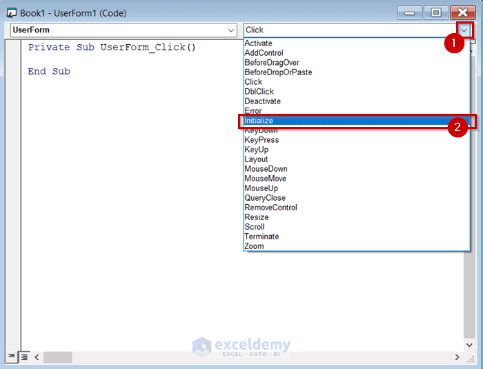
Another Private Sub Procedure named UserForm_Initilizer() will be created.
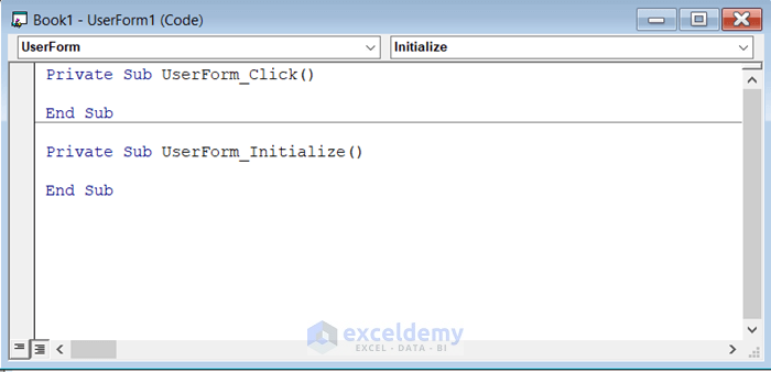
- Delete the first Private Sub and enter the following code:
Private Sub UserForm_Initialize()
Me.ListBox1.AddItem "Name"
End Sub
Code Breakdown
- We create a Private Sub procedure named UserFprm_Initializer().
- We use the Me object, which acts as an implicitly declared variable.
- We use the AddItem method to make a list of values displayed by ListBox1.
- We end the Sub Procedure.
- Double-click on the CommandButton on the UserForm.
Another Private Sub Procedure named CommmandButton1_Click() will be created.
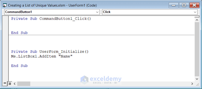
- Enter the following code in the UserForm1 box:
Private Sub CommandButton1_Click()
Dim unq_val As New Collection
Dim a As Integer
Dim i As Long
For a = 2 To 4
For i = 6 To Sheets(a).Range("B" & Rows.Count).End(xlUp).Row
On Error Resume Next
unq_val.Add Sheets(a).Cells(i, "B"), Sheets(a).Cells(i, "B")
Next i
Next a
For Each itm In unq_val
Me.ListBox1.AddItem itm
Next itm
End Sub
Private Sub UserForm_Initialize()
Me.ListBox1.AddItem "Name"
End Sub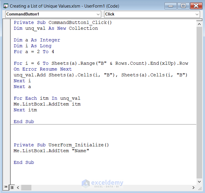
Code Breakdown
- We create a Private Sub Procedure named CommandButton1_Click().
- We declare a variable unq_val as New Collection.
- We declare another variable a as Integer.
- We declare i as long.
- We use a For Next loop to take values from multiple worksheets.
- In the For Next Loop, we nest another For Next loop to get values from different cells.
- We use the Add Sheets method to get the unique values from the cells in Excel sheet.
- We use the For Each Next loop to add the unique values in the ListBox.
- We end the Sub Procedure.
- Save the code and go back to the worksheet.
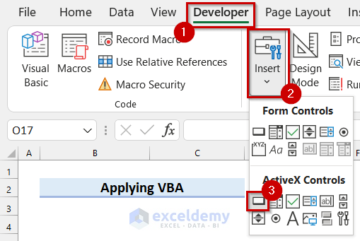
- Go to the Developer tab.
- Select Insert.
- Select CommandButton from ActiveX Controls.
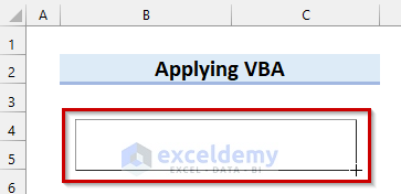
- Click and drag your mouse cursor where you want the CommandButton.
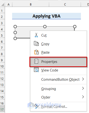
- Right-click on the CommandButton.
- Select Properties.
- Change the Properties if you like. I changed my caption to Show UserForm.
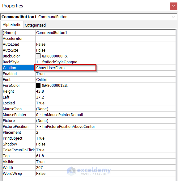
The caption of the CommandButton is changed.
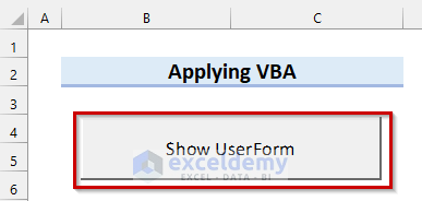
A Module with a Private Sub will appear.
- In that Module enter the following code:
Private Sub CommandButton1_Click()
UserForm1.Show
End Sub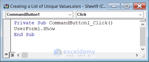
Code Breakdown
- We create a Private Sub Procedure named CommandButton1_Click().
- We use the Show method to show the UserForm1.
- We end the Sub Procedure.
- Save the code and go back to your worksheet.
- Click on Show UserForm.
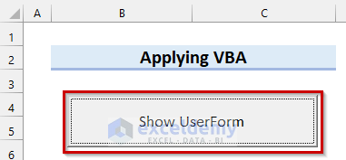
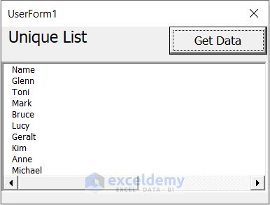
The UserForm will appear.
- Click on the CommandButton.

The list of unique values from multiple sheets in Excel is displayed.
Things to Remember
- Whenever working with Visual Basic, the workbook should be saved as Excel Macro-Enabled Workbook.
Download Practice Workbook
<< Go Back to Learn Excel
Get FREE Advanced Excel Exercises with Solutions!


Could you give a bit more information on the Add Sheets method to get the unique values from the cells in Excel sheet please.
Hello Lodewijk,
I suppose you want to know more about the Power Query Editor and how it can add sheets to get unique values.
Power Query Editor is very useful in the case of data preparation.
To use this editor, you have to use the Get Data feature from the Data tab. You can get data from different kinds of files such as Excel workbooks, PDFs, Text, etc. Then, you can transform those datasets using the operator available. Here, we removed rows from the tables. You can also combine different tables from those files by the Append or Merge operator. The Append operator is used to create a new query having all the rows from the datasets and the Merge operator is used to have a query with all the columns. You have to use the Append operator to get the unique values. Finally, you can load the query in the existing worksheet or a new worksheet.
If you face any further problems, please share your Excel file with us in the comment section.
Regards
Arin Islam,
Exceldemy.