Method 1 – Use VALUE Function
Steps:
- Choose a cell (F5) and write the following formula down-
=VALUE(D5)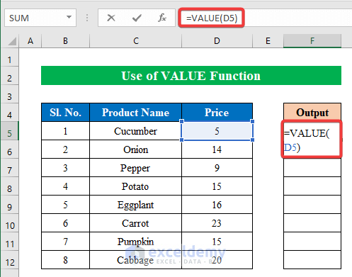
- Press ENTER and drag the Fill Handle down to fill all the cells.
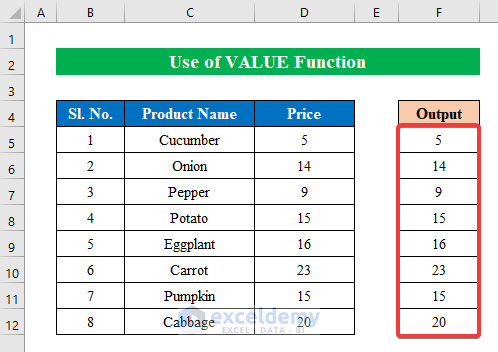
- The cells (F5:F12) are selected press CTRL+1 from the keyboard.

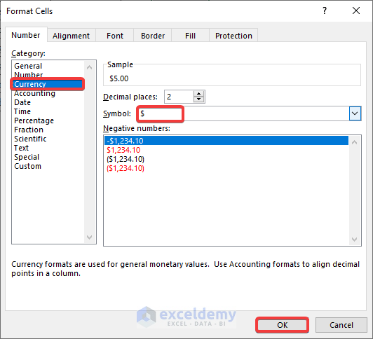
- A new window will appear named “Format Cells”.
- From the new window choose “Currency” and your desired symbol from the “Symbol” box.
- Hit OK to continue.
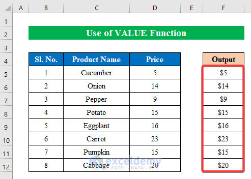
- Get the currency format in a new column within the blink of an eye.
Method 2 – Utilize Paste Special Tool
Steps:
- Choose cells (D5:D12) and click CTRL+C to copy.
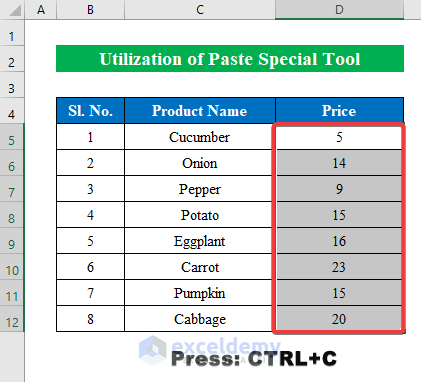
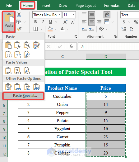
- Click “Paste Special” from the Home ribbon.
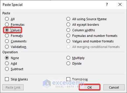
- A new dialog box will appear named “PasteSpecial”.
- The dialog box choose “Values” and press OK to change all the cell values to numeric values.
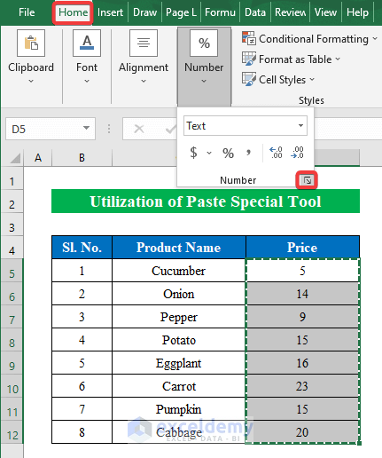
- Change the cell format to currency format.
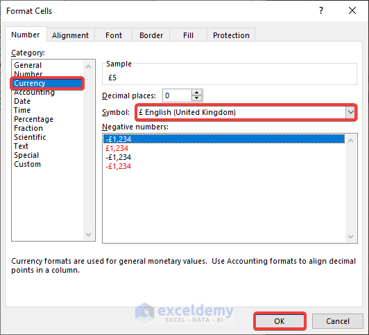
- Select the cells (D5:D12) and click the “FormatCells” icon from the Home ribbon.
- Click “Currency” and choose your desired currency symbol in the “Symbol” box.
- Hit OK to finish.
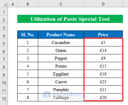
- Our problem and now the currency format is displayed for the chosen cells.
Method 3 – Use Format Cells Feature
Steps:
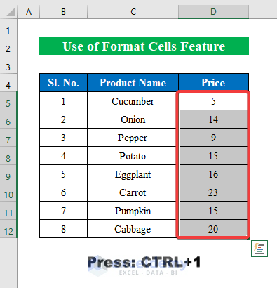
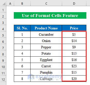
- Choose cells (D5:D12) and press CTRL+1 from the keyboard to go to the “Format Cells” window.
- Choose “Currency” and your choice of currency format from the drop-down list of “Symbol”.
- Press OK.
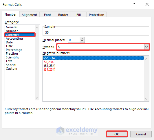
- Get the currency format for the cells within a moment solving our problem.
Download Practice Workbook
Download this practice workbook to exercise while you are reading this article.
Related Articles
- List of Currency Symbols in Excel
- How to Convert Currency to Number in Excel
- Convert Currency to Words in Excel
- Currency with 2 Decimal Places in Excel
<< Go Back to Currency Format | Number Format | Learn Excel
Get FREE Advanced Excel Exercises with Solutions!


Thank you for the several means to solve this problem. I tried all but the currency sign didn’t still appear. What could possibly be the problem?
Dear Anita,
Thank you for the comment. We really appreciate your response for sharing with us.
The currency sign not appearing in Excel may be due to the values are stored as text in your spreadsheet. When values are stored as text, you need to convert those as numbers and then change the format to currency to get your desired currency format. You can follow the below instructions to learn about this technique.
First, choose the cells (D5:D12) and click the error icon following the image below.
Next, choose Convert to Number option from the list.
As the numbers are now converted as number, now press CTRL+1 to visit the Format Cells feature to add currency symbol.
From the Format Cells window, choose Currency from the left pane, select your desired currency symbol and hit OK.
As a result, you will get the currency sign added in your worksheet.
If you are still having problem with the currency symbol, then you can share your workbook with us. We will check and solve the problem.
Thanks & Regards
Wasim Akram
Team Exceldemy