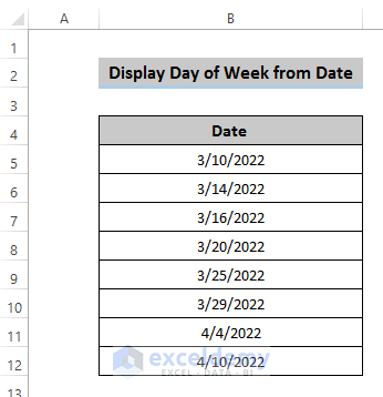
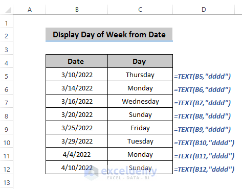
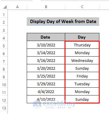
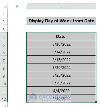
Here’s a simple dataset of some dates that we’ll convert into days of the week.
Method 1 – Using the TEXT Function to Display the Day of the Week from a Date in Excel
Steps
- Select cell C5.
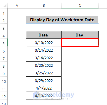
- Apply the following formula:
=TEXT(B5,"dddd")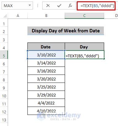
Note:
You can use two variations:
- TEXT(B5,”dddd”) : This formula will show the entire day’s name in the result cell which means if you apply ‘dddd’ in the formula box, it will provide you the full day name.
- TEXT(B5,”ddd”): This will provide a short version of your required day.
- Press Enter to apply the formula.
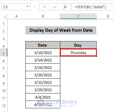
- Double-click on the Fill Handle icon to fill the column.
Method 2 – Displaying the Day of the Week from a Date with Format Cells
Steps
- Copy all the dates and paste them into column C.
- Select all the dates in column C.
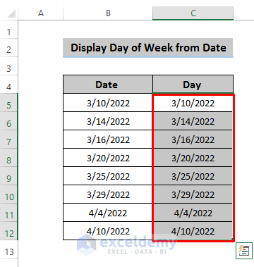
- Go to the Home tab and, from the Number group, select the dialog box launcher in the corner. Alternatively, right-click on the cell and select Format Cells from the Pop-up menu or press Ctrl + 1.

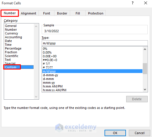
- A Format Cells dialog box will appear. Select the Number option and, in the Category section, select Custom.
- In the Type section, type ‘dddd’ for the whole day name or ‘ddd’ for the short name.
- Click on ‘OK’.
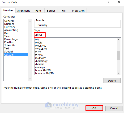
- We get dates converted into days of the week.
Method 3 – Inserting the WEEKDAY Function to Display the Day of the Week from a Date
Steps
- Select cell C5 where you want to apply your WEEKDAY function.
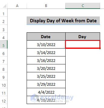
- In the formula box, insert the following formula:
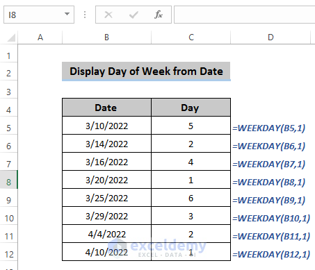
=WEEKDAY(B5,1)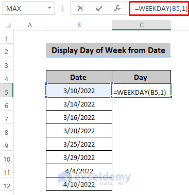
- Press Enter to apply the formula. Since we put 1 in the return_type parameter so, starts the week from Sunday. So, value 5 denotes Thursday.
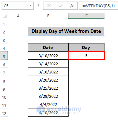
- Double-click on the Fill Handle icon to apply the formula for all the dates.
Method 4 – Combining WEEKDAY and CHOOSE Functions to Display the Day of the Week
Steps
- Select cell C5 where you want to apply the formula.
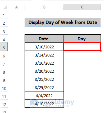
- Insert the following formula in the formula box.
=CHOOSE(WEEKDAY(B5),"Sun","Mon","Tue","Wed","Thu","Fri","Sat")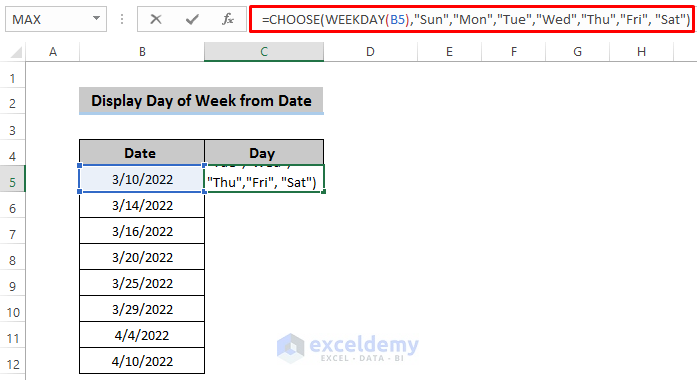
- Press Enter to apply this formula.
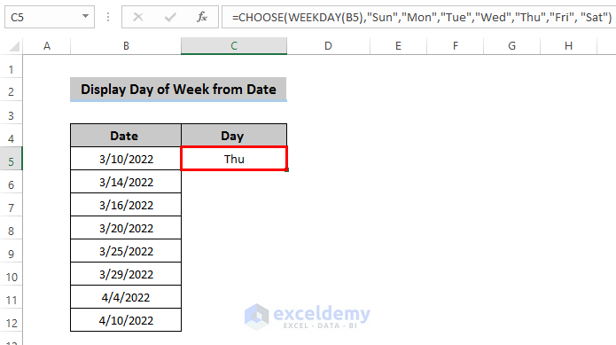
- Drag the Fill Handle icon or double-click on the icon to apply this down the column.
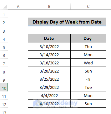
Breakdown of the Formula
The WEEKDAY function provides the number of the corresponding days. By default, it starts on Sunday and the last day of the week is Saturday.
The CHOOSE function selects the string from your given string array based on the input. In our work, the WEEKDAY function returns 5 for the first date, and the CHOOSE function converts it into ‘Thu’ which is the shorter version of Thursday.
Method 5 – Joining SWITCH with the WEEKDAY Function to Show Days of the Week
Steps
- Select cell C5 to apply the formula.
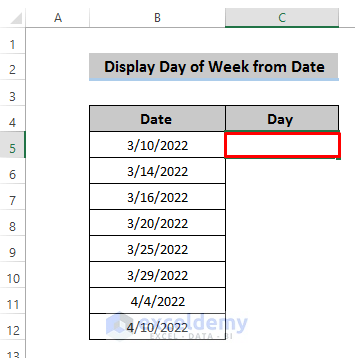
- In the formula box, insert the following formula
=SWITCH(WEEKDAY(B5,1),1,"Sun",2,"Mon",3,"Tue",4,"Wed",5,"Thu",6,"Fri",7,"Sat")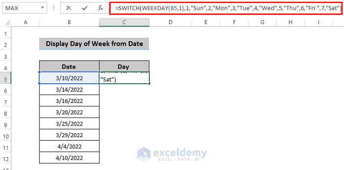
- Press Enter to apply the formula.
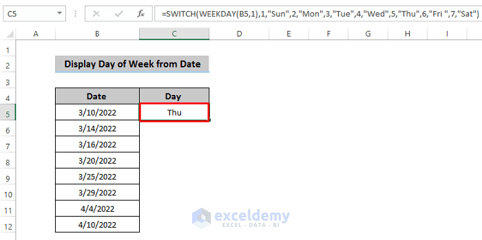
- Drag the Fill Handle icon down the column or double-click on the icon.

Breakdown of the Formula
The WEEKDAY function provides the number of the corresponding days. By default, it starts on Sunday and the last day of the week is Saturday.
The SWITCH function selects the string from the string list based on the value of the first argument, which is the WEEKDAY function in the sample.
Method 6 – Showing Days of the Week in Excel Using the Long Date Format
Steps
- Copy the dates of column B into column C and select all the cells from column C.
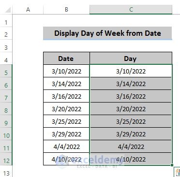
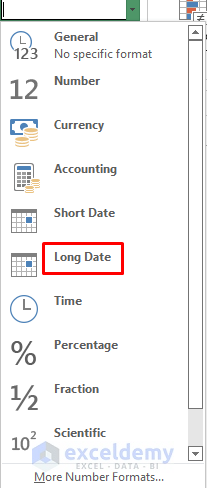
- Go to the Home tab. Click on the drop-down box in the Number group.

- In the drop-down menu, select Long Date.
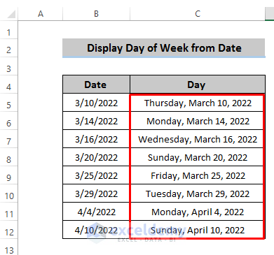
- This will change all the dates into the Long Date format.
Method 7 – Using Excel Power Query to Display the Day of the Week from a Date
Steps
- Select the dataset.
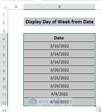
- Go to the Data tab in the ribbon and select From Table/Range.

- Click on ‘OK’ after putting in the dataset range.
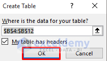
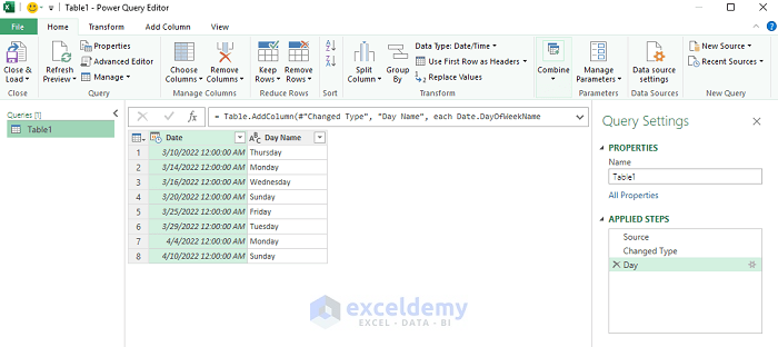
- This will open the Power Query editor.
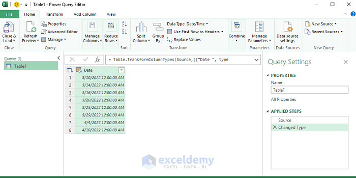
- If your dataset isn’t in the date type, go to the Add Column tab and, from the Date & Time section, select Date.
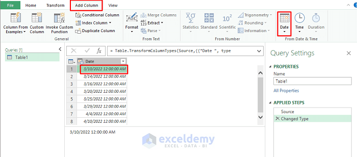
- In the Date option, select Name of Day from Day.
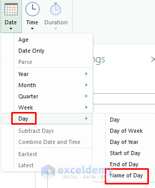
- This will create a new column to show the days of the week.
- Click on Save & Load.
Method 8 – Displaying the Day of the Week from a Date with a Pivot Table
Case 8.1 – Combining WEEKDAY and SWITCH Functions
Steps
- Select the range of cells B4:B12.
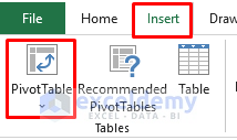
- Go to the Insert tab and select PivotTable from the Tables group.
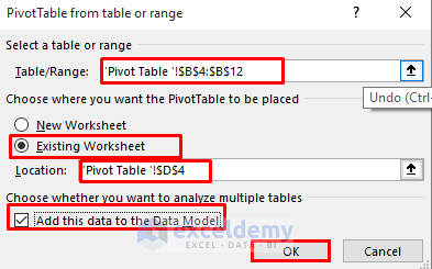
- In the PivotTable dialog box, select your data table range, choose Existing Worksheet to place the PivotTable, and click on Add this data to the Data Model.
- Click OK.
- The PivotTable Fields will appear on the right side of the worksheet.
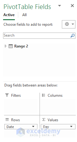
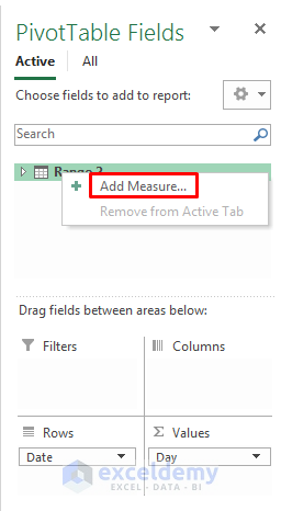
- Right-click on Range 2 of PivotTable Fields and select Add Measure.
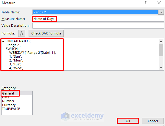
- This will open the Measure dialog box where you can create the DAX measure. Set the Category as General and input a Measure Name.
- Insert the following formula in the DAX Formula box and click on OK.
=CONCATENATEX (
    'Range 2',
    SWITCH (
        WEEKDAY ( 'Range 2'[Date], 1 ),
        1, "Sun",
        2, "Mon",
        3, "Tue",
        4, "Wed",
        5, "Thu",
        6, "Fri",
        7, "Sat"
    ),
    ", "
)
- Here’s the result.
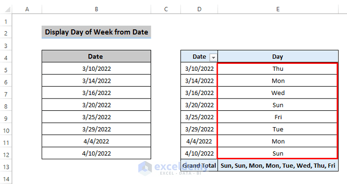
Case 8.2 – Using the FORMAT Function
Steps
- Make the pivot table just like the previous case.
- Right-click on Range 3 in the PivotTable Fields and select Add Measure.
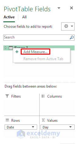
- Insert the following formula in the DAX formula box and click on ‘OK’
=CONCATENATEX('Range 3',FORMAT('Range 3'[Date],"dddd"),",")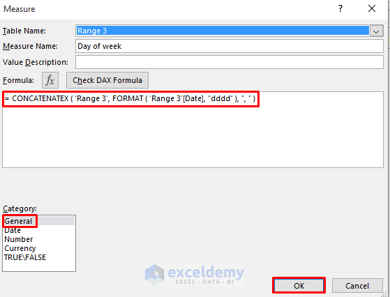
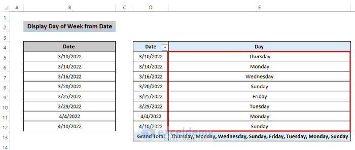
- Here’s the output.
Download the Practice Workbook
<< Go Back to Date and Time | Split | Learn Excel
Get FREE Advanced Excel Exercises with Solutions!


This has been super super helpful, merci buckets..,
Hello Kristi,
You are most welcome.
Regards
ExcelDemy