Dynamic Named Range Based on Cell Value in Excel

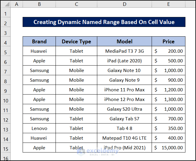
The basic idea of naming a range is the simple — we will use the Name Manager from the Formula tab. For each method, we are going to use the same dataset.

Method 1 – Create a Dynamic Named Range Based on Cell Value with the OFFSET Function

Steps:

• Go to the Formulas tab on your ribbon.
• Select Name Manager from the Defined Names group section.

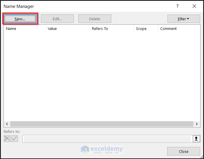
• The Name Manager box will appear.
• Click on the New button in the top-left corner of the box.

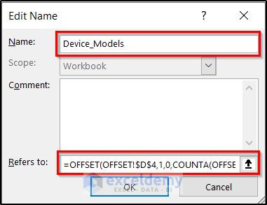
• Insert a name in the Name field of the Edit Name.  We are choosing Device_Models as the name.
• In the Refers to field, insert the following formula:

• Click on OK and close the Name Manager.  The naming of the range is now complete.
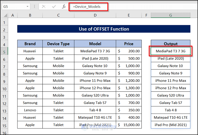
• Go to the spreadsheet and type out the following.

• Press Enter. You will find that the range will appear.

• If we add a value now, it will automatically update the output.

Read More: OFFSET Function to Create & Use Dynamic Range in Excel

Method 2 – Combine OFFSET and MATCH Functions to Create a Dynamic Named Range

Steps:

• Go to the Formulas ribbon on your tab.
• Select Name Manager from the Defined Names group section.

• When the Name Manager box pops up, select New in the top-left corner of the box.

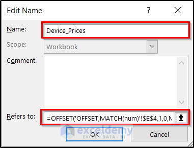
• Fill the Name field with the name you want.
• Insert the following formula in the Refers to field beneath:

• Click on OK and close the Name Manager.  The dynamic named range based on cell value is now complete.
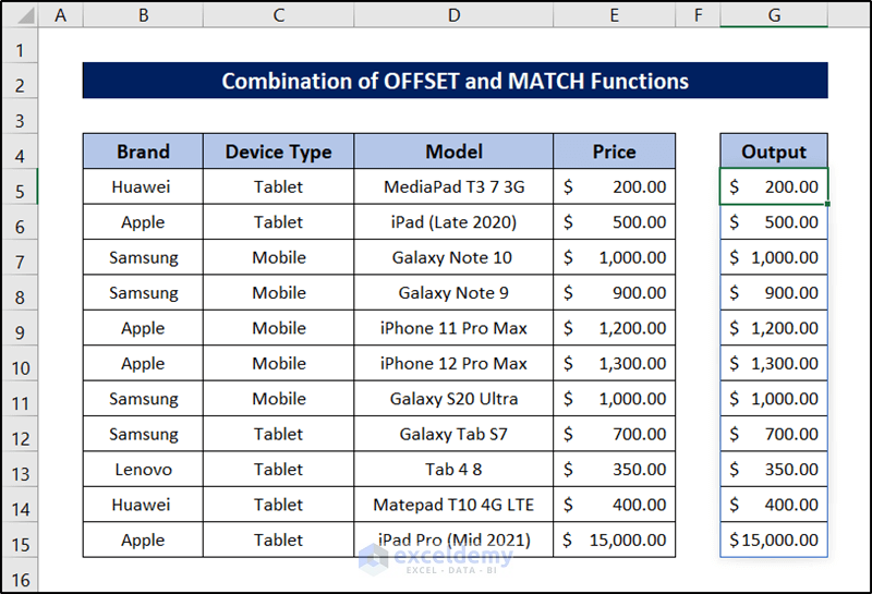
• Let’s go back to the Excel spreadsheet and insert the following formula.

• Press Enter.

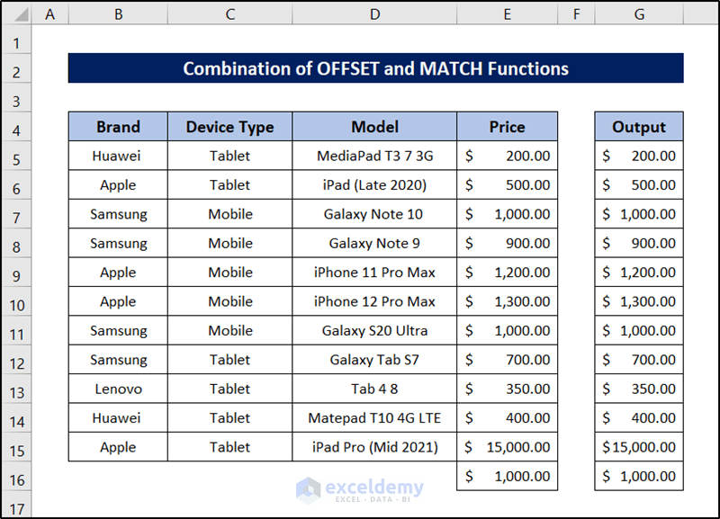
• Insert a value under the column and you will see the output change accordingly.

Read More: Dynamic Range for Multiple Columns with Excel OFFSET

Method 3 – Generate a Named Range for Text Values by Joining OFFSET and MATCH Functions

Steps:

• Go to the Formulas tab on your ribbon.
• Select Name Manager from the Defined Names group section.

• Click on the New button on the top-left of the dialog box.

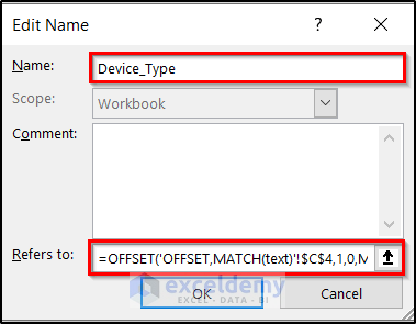
• Enter a name in the Name field in the following box, such as Device_Type.
• Insert the following formula in the Refers to field to define the range.

• Click on OK and close the Name Manager.
• To test it out, go back to the spreadsheet and use the following in a cell.

• Press Enter.

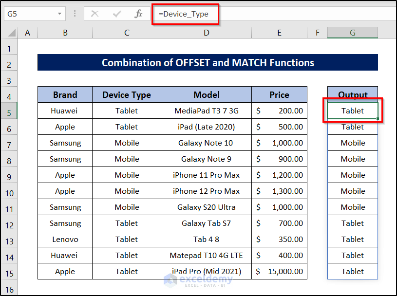
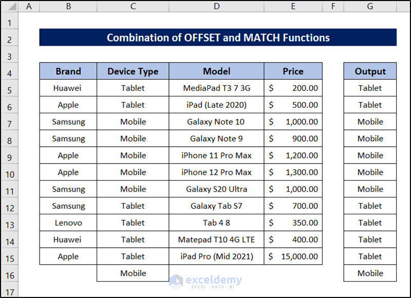
• Enter a value under the column we are filtering from, and the output should change accordingly.

Method 4 – Apply the FILTER Function to Create a One-Dimensional Dynamic Named Range in Excel

Steps:

• Go to the Formulas tab on your ribbon.
• Select Name Manager from the Defined Names group section.

• Click on the New button on the top-left of the Name Manager box that will pop up next.

• Insert the name in the Name field of the following box.
• Insert the formula in the Refers to box as the reference.

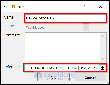
• After clicking on OK here, close the Name Manager box.
• To test the range out, type out or copy the name you gave to the range in a formula bar (after an equals sign).
• Press Enter.

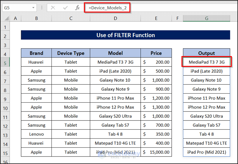
• Insert something under the column we are picking the reference from, and it will update the output.

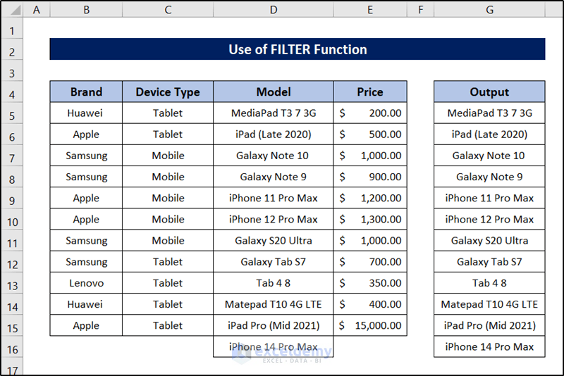
Method 5 – Create a Two-Dimensional Dynamic Named Range in Excel

Steps:

• Go to the Formulas tab on your ribbon.
• Select Name Manager from the Defined Name group section.

• Click on New from the top-left of the Name Manager box that pops up.

• Insert a name in the Name field for the range.
• Insert the following formula in the Refers to field below.

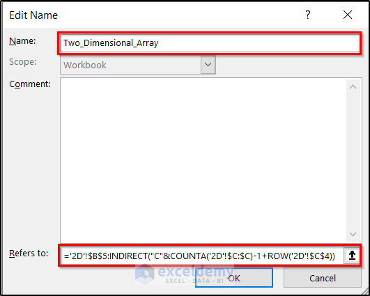
• Click on OK and close the Name Manager box.
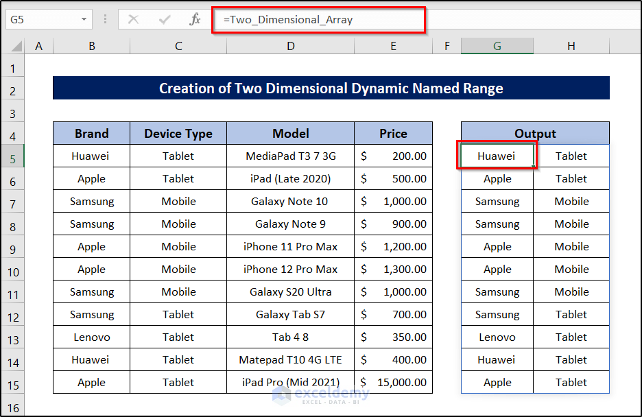
• To test if the formula works, go back to the spreadsheet and use the range’s name in a cell:

• After pressing Enter, you will find something like this.

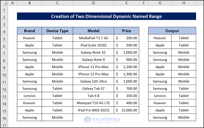
• Insert two values under the two columns we are taking for the two-dimensional arrays. The table should update the result.

Read More: Create Dynamic Sum Range Based on Cell Value in Excel

Insert the INDEX Function in Excel for Creating a Named Range Based on Cell Value

Steps:

• Select the Formulas tab and go to Name Manager, which you can find from the Defined Names group.

• Click on the New button at the top left of the popped-up box.

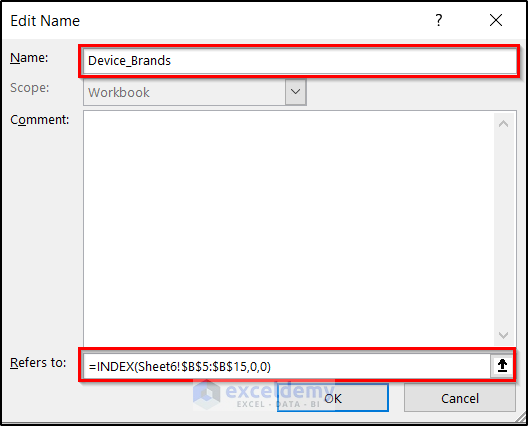
• Insert a name in the Name box.
• Insert the following formula in the Refers to field below that.

• Click on OK.
• Close the Name Manager box also.
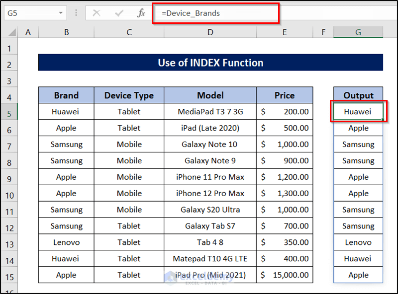
• Go back to the spreadsheet and insert the name of the range in a formula.

• Press Enter on your keyboard.

Read More: How to Create Dynamic Range Using Excel INDEX Function

Use Name Cell in Excel to Generate Named Range

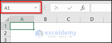
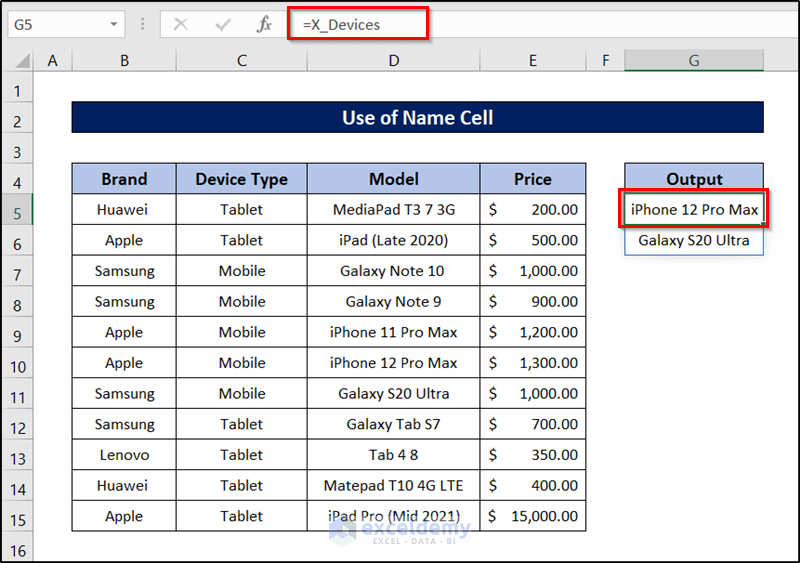
The simplest way to create a named range is to use the Name Cell feature of Excel. You can find it on the left side of the formula box on the spreadsheet.

Steps:

• Select the range you want to name and manually edit this.

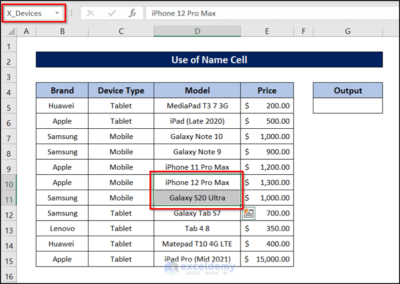
• If you want to reference the range, just use the name you have given it.

Define Names from a Selected Range

Steps:

• Select a range.

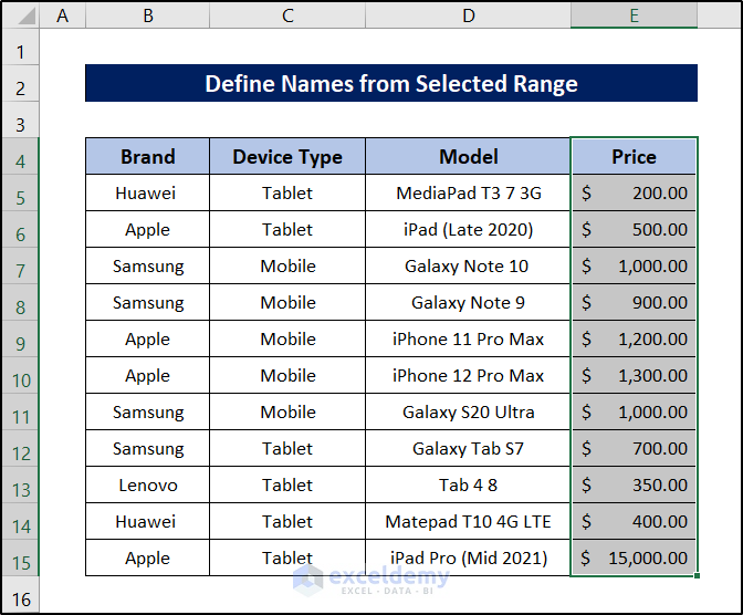
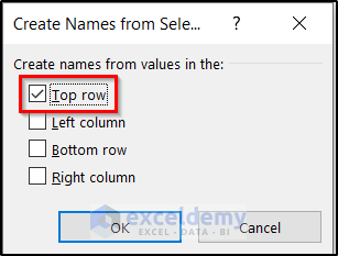
• Select the Create from Selection feature from the Defined Names group of the Formulas tab.

• Select the option that matches your criteria. In this case, it is the Top row.

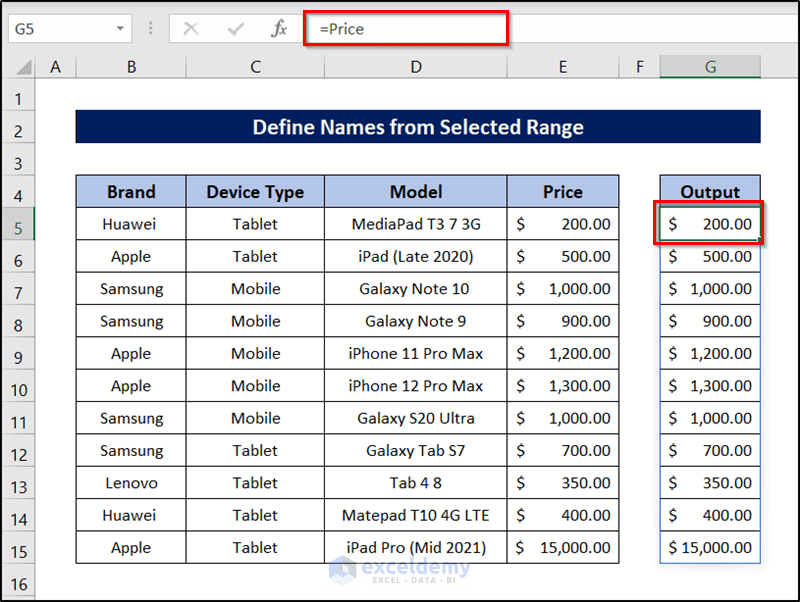
• You can find the range through the name of the top row as shown in the following figure.

Download the Practice Workbook

Further Readings

• Data Validation Drop Down List with Excel Table Dynamic Range
• How to Create a Range of Numbers in Excel

<< Go Back to Dynamic Range | Named Range | Excel Formulas | Learn Excel