Find And Replace Multiple Values in Excel (6 Quick Methods)

Method 1 – Use the Find and Replace Tool for Multiple Values in Excel

Case 1 – Find and Replace Text Values

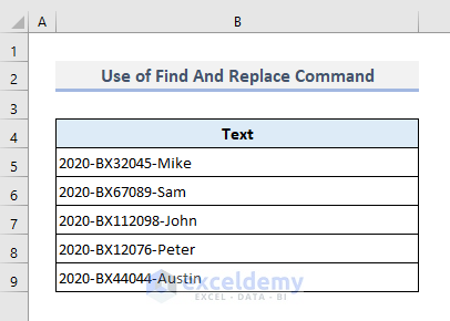
In the table below, we want to replace the value ‘2020’ with ‘2021’ in all cells.

Steps:

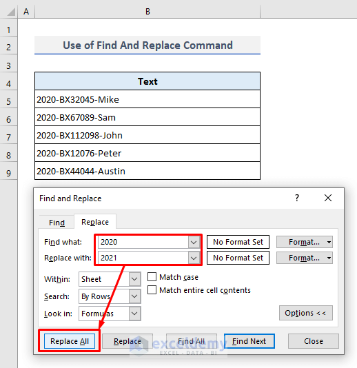
• Press Ctrl + H, and the Find and Replace dialog box will open up.
• Type ‘2020’ in the Find what box.
• In the Replace with box, type ‘2021’.
• Click on the Replace All button.

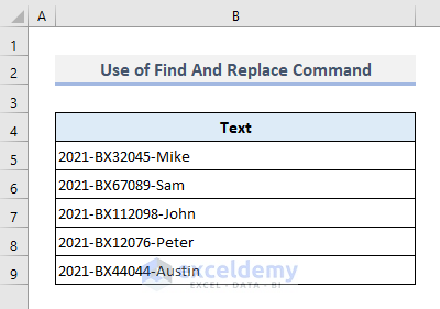
• The function changes all the instances of 2020 with 2021 throughout the sheet.

Case 2 – Find and Replace with “?” for Wild Characters

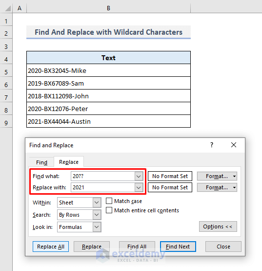
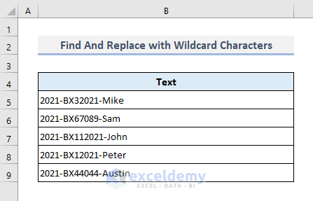
We have different numeric values at the beginning of the following texts, but all of them have a specific format ‘20XX’. The last two digits will be replaced with ‘21’.

Steps:

• Press Ctrl + H to open the Find and Replace dialogue box.
• In the Find what box, type ‘20??’.
• Input the value ‘2021’ in the Replace with box.
• Press Replace All and you’re done.

• You’ll see the following outputs immediately.

Case 3 – Find and Replace Formulas

We have some sales data for 5 days. Cell C11 contains the total value, but we want to find out the average of the sales data there.

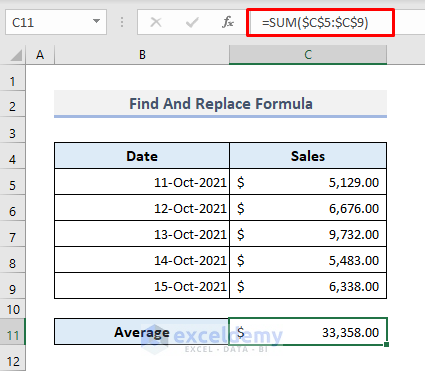
Steps:

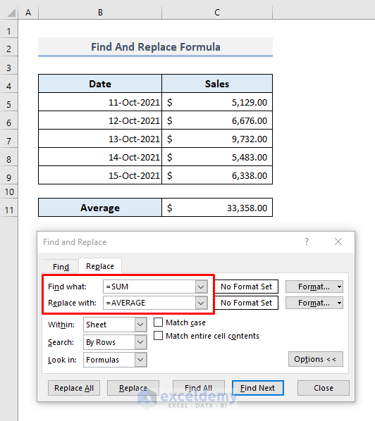
• Open the Find and Replace dialog box.
• In the Find what box, type ‘=SUM’.
• Copy ‘=AVERAGE’ in the Replace with box.
• Press Find Next and click on the Replace button.

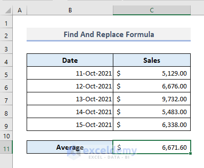
• In the output Cell C11, you’ll get the new calculated result.

Read More: How to Find and Replace Using Formula in Excel

Case 4 – Find And Replace Cell Formats

In the following table, there are some rows with a specific color. We’ll replace the color with another one, let’s say green.

Steps:

• Open the Find and Replace dialog box.
• In front of the Find what box, click on the Format option and select the color that has been used in the cells in the table.
• Click on the second Format tab and choose the new color.
• Press Replace All.

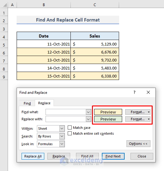
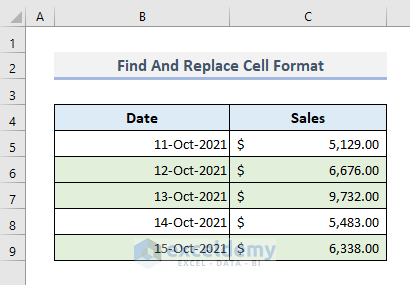
• All the applicable cells will be reformatted.

Read More: How to Find and Replace Text Color in Excel

Method 2 – Insert the REPLACE Function to Find and Replace Multiple Values in Excel

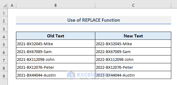
In the following picture, the column with the New Text header will display the modified texts.

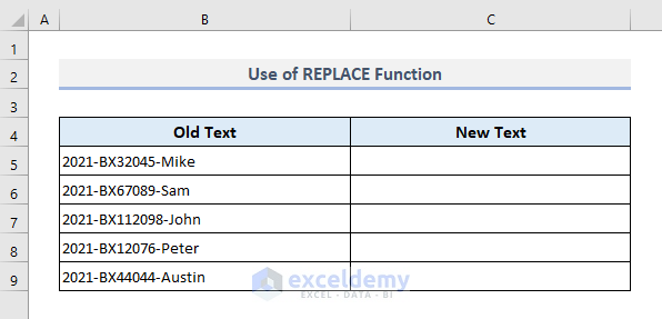
• In the first output Cell C5, the required formula with the REPLACE function will be:

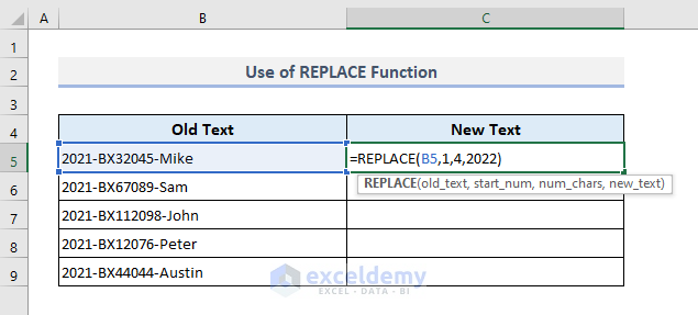
• Press Enter and use Fill Handle to autofill the rest of the cells, and you’ll get the new text values. We have replaced the values ‘2021’ with ‘2022’ for all texts.

Read More: How to Find and Replace in Excel Column

Method 3 – Apply a Nested SUBSTITUTE Formula to Find and Replace Multiple Values

In the following picture, Column B has some random text data. The table on the right represents the values that have to be replaced with the new ones.

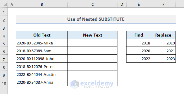
• In the first output Cell C5, the formula will be:

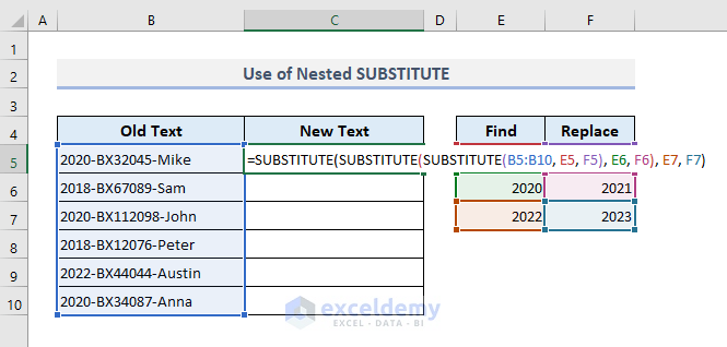
• Press Enter and you’ll get an array with the new text values.

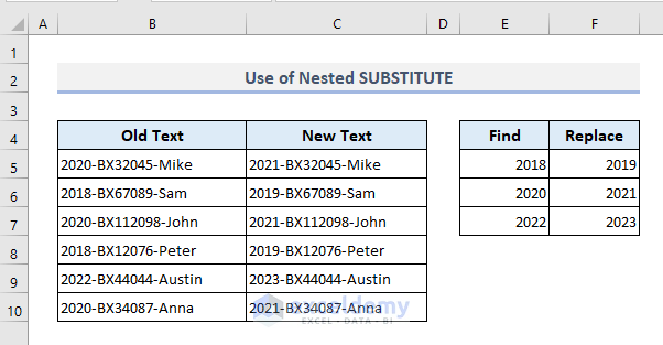
How Does the Formula Work?

• The innermost SUBSTITUTE function replaces the value ‘2018’ with ‘2019’.
• The second SUBSTITUTE function looks for ‘2020’ and replaces it with ‘2021’.
• The outer SUBSTITUTE function searches ‘2022’ and substitutes it with ‘2023’.

Method 4 – Use the XLOOKUP Function to Search and Replace Multiple Values in Excel

If you’re an Excel 365 user, you can also use the XLOOKUP function.

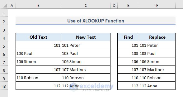
In the following dataset, there are some text values in the Old Text column. The second table on the right represents data that needs to be searched for and replaced. If the function can’t find the given values, then the old content will remain.

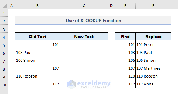
• The required formula in the first output Cell C5 should be:

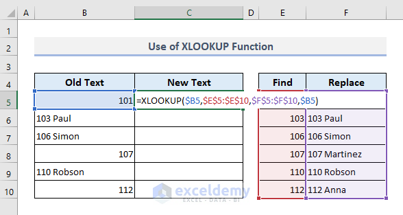
• Press Enter and auto-fill the entire column.

Method 5 – Combine IFNA and VLOOKUP Functions to Find and Substitute Multiple Values

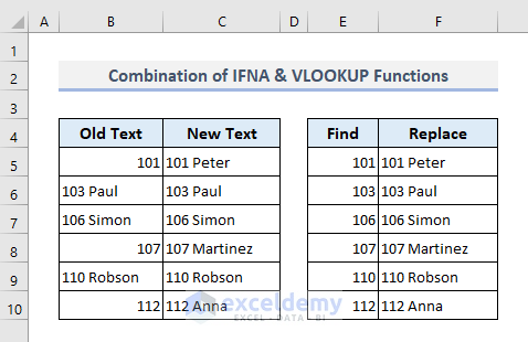
• The required formula in the output Cell C5 will be:

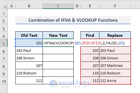
• After pressing Enter and filling down the rest of the cells in Column C, we’ll get all the new text data as shown in the picture below.

Method 6 – Embed VBA Code to Make a UDF to Find and Replace Multiple Values

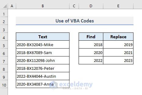
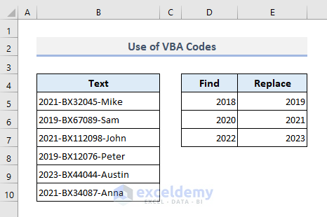
In the following dataset, the text values in Column B will be modified by replacing the numeric values at the beginning. These values are in the table on the right.

Steps:

• Right-click on the Sheet name.
• Select the option ‘View Code’. A VBA window will appear.
• Paste the following codes there:

Option Explicit
Sub FindnReplaceMultipleValues()
  Dim Rng As Range
  Dim OldText As Range
  Dim ReplaceData As Range
  On Error Resume Next
  Set OldText = Application.InputBox("Select Old Text Range:", "Find And Replace Multiple Values", Application.Selection.Address, Type:=8)
  Err.Clear
  If Not OldText Is Nothing Then
    Set ReplaceData = Application.InputBox("Replace What And With:", "Find And Replace Multiple Values", Type:=8)
    Err.Clear
    If Not ReplaceData Is Nothing Then
      Application.ScreenUpdating = False
        For Each Rng In ReplaceData.Columns(1).Cells
          OldText.Replace what:=Rng.Value, replacement:=Rng.Offset(0, 1).Value
        Next
      Application.ScreenUpdating = True
    End If
  End If
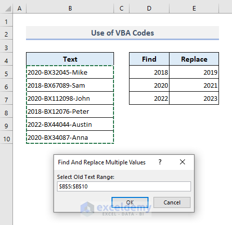
End Sub

• Press F5 and a dialogue box as shown in the screenshot below will appear.
• Select the old cells that you have to modify and press OK.

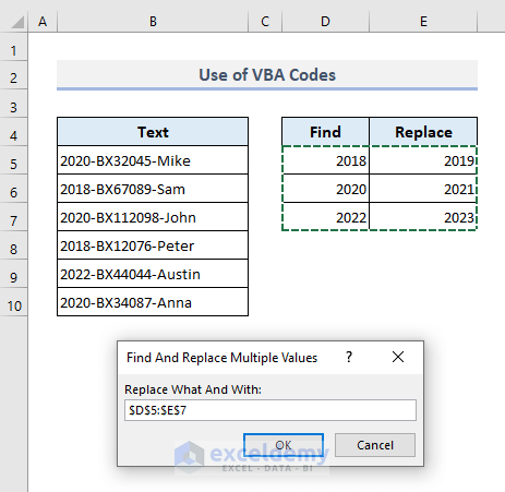
• A second dialog box will open. Select the entire table range (D5:E7) on the right.
• Press OK.

• You’ll see the new and modified texts in Column B under the Text header.

Download the Practice Workbook

Related Articles

• How to Find and Replace Asterisk (*) Character in Excel
• Find and Replace Tab Character in Excel
• [Fixed!] Excel Find and Replace Not Working
• How to Replace Special Characters in Excel
• How to Substitute Multiple Characters in Excel

<< Go Back to Find and Replace | Learn Excel