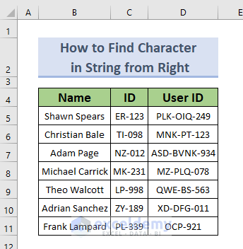
The sample dataset contains information for a group of people who work in an office and have their own ID and User ID.
Method 1 – Using Excel RIGHT Function to Find Character in String from Right
The simplest way to find the characters in a string from the right is to use the RIGHT function.
Steps:
- Make a new column and enter the following formula in cell E5.
=RIGHT(C5,3)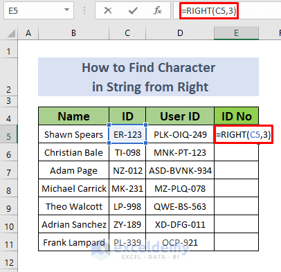
The RIGHT function takes the character string in cell C5 and finds the last 3 characters from it. As each ID has 3 numbers, we put [num_chars] as 3.
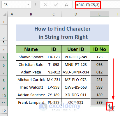
- Hit the ENTER button and the last 3 digits of the ID are returned in cell C5.

- Use the Fill Handle to AutoFill lower cells.
Read More: How to Find Character in String Excel
Method 2 – Applying Excel LEN and FIND Functions to Extract Character in String from Right
In this example we want to extract the surnames from the names column.
Steps:
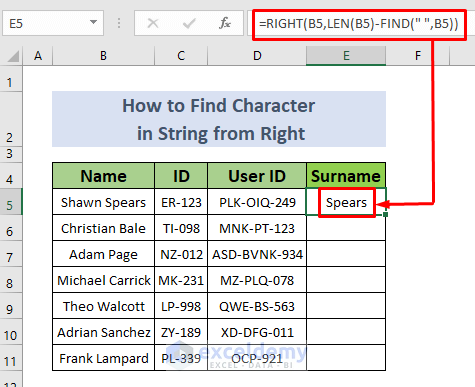
- Make a new column for surnames and enter the following formula in cell E5.
=RIGHT(B5,LEN(B5)-FIND(" ",B5))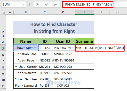
The Find function will identify the position of the Space between first name and surname and the Len function determines the length of the string.
The RIGHT function identifies which characters should be stored in cell E5.
- Press the ENTER button and you will see the surname of cell B5 in cell E5.
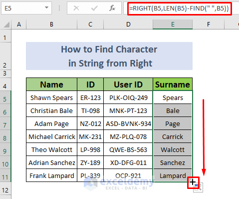
- Use the Fill Handle to AutoFill lower cells.
Read More: How to Find from Right in Excel
Method 3 – Utilizing Combined Functions to Find Character in String from Right
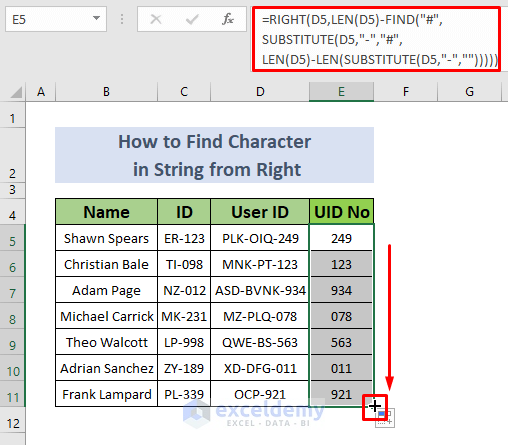
Nesting the LEN, FIND and SUBSTITUTE functions into the RIGHT function allows us to find the User ID.
Steps:
- Make a new column for User ID No and enter the following formula in cell E5.
=RIGHT(D5,LEN(D5)-FIND("#",SUBSTITUTE(D5,"-","#",LEN(D5)-LEN(SUBSTITUTE(D5,"-","")))))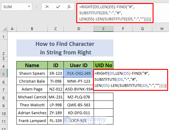
Formula Breakdown
- LEN(D5)—-> The Length function returns the number of characters.
- Output: 11
- SUBSTITUTE(D5,”-“,””)—-> The SUBSTITUTE function replaces the hyphens with nothing.
- SUBSTITUTE(“PLK-OIQ-249″,”-“,””)—-> becomes PLKOIQ249
- Output: “PLKOIQ249”
- LEN(SUBSTITUTE(D5,”-“,””))—-> becomes LEN(“PLKOIQ249”)
- Output: 9
- LEN(D5)-LEN(SUBSTITUTE(D5,”-“,””)))—-> becomes LEN(D5)-LEN(“PLKOIQ249”)
- 11-9
- Output : 2
- SUBSTITUTE(D5,”-“,”#”,LEN(D5)-LEN(SUBSTITUTE(D5,”-“,””))—-> becomes
- SUBSTITUTE(D5,”-“,”#”,2)—> It substitutes the 2nd hyphen ‘-’ with hashtag ‘#’)
- Output: “PLK-OIQ#249”
- FIND(“#”,SUBSTITUTE(D5,”-“,”#”,LEN(D5)-LEN(SUBSTITUTE(D5,”-“,””))))—-> becomes
- FIND(“#”,”PLK-OIQ#249″)—-> The FIND function finds the position of the given character #.
- Output: 8
- RIGHT(D5,LEN(D5)-FIND(“#”,SUBSTITUTE(D5,”-“,”#”,LEN(D5)-LEN(SUBSTITUTE(D5,”-“,””)))))—-> turns into
- RIGHT(D5,LEN(D5)-8)—->
- RIGHT(D5,11-8)—->
- RIGHT(D5,3)—->
- RIGHT(“PLK-OIQ-249”,3)—-> The RIGHT function extracts the number of characters from the right side.
- Output: 249
The User ID 249 is returned.
- Hit ENTER and you will only see the number in the User ID.
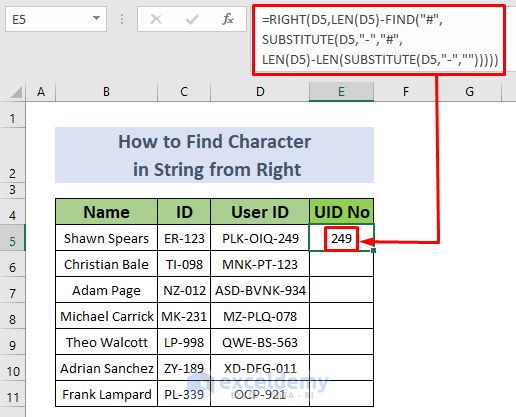
- After that, use the Fill Handle to AutoFill lower cells.
Read More: How to Find Text in Cell in Excel
Method 4 – Finding Characters in String from Right Using Flash Fill
Steps:
- Make a new column for surnames and enter the surname (Spears) in cell B5.
- Select Home >> Fill >> Flash Fill
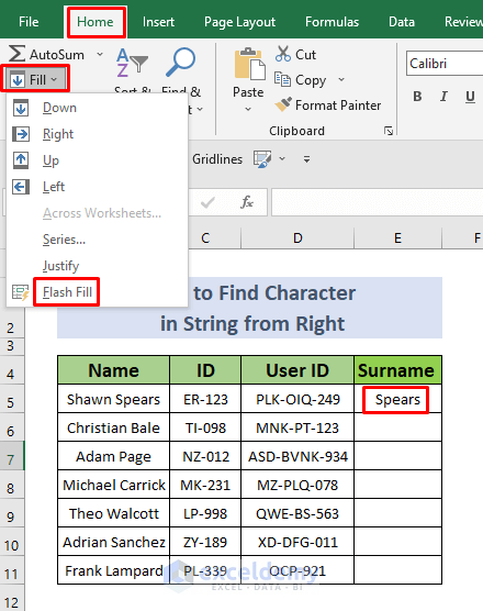
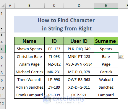
The Flash Fill command follows a pattern. It detects the character string Spears as the right-sided characters of the whole string in cell B5 and will do the same for other cells.
- This operation will return all the surnames in the remaining cells E6 to E11.
Read More: How to Check If Cell Contains Specific Text in Excel
Download Practice Workbook
Related Articles
- Excel Find Last Occurrence of Character in String
- How to Find If Range of Cells Contains Specific Text in Excel
- How to Find * Character Not as Wildcard in Excel
<< Go Back to Find in String | String Manipulation | Learn Excel
Get FREE Advanced Excel Exercises with Solutions!

