We have a sample dataset that contains Sales Person and Sales information. We will find a name from the column named Sales Person and return the row number of that string.
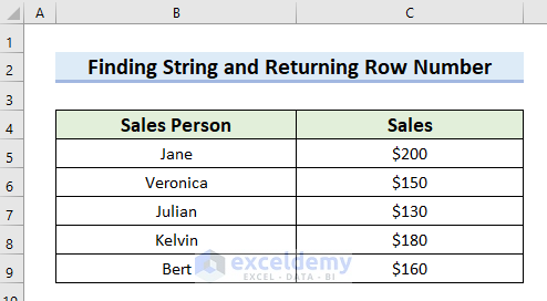
Method 1 – Using the MATCH Function to Find a String in a Column and Return the Row Number in Excel
We will find the string that is in cell E5 from the column named Sales Person and return the row number in cell F5.
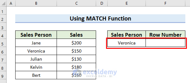
Steps:
- Select the cell where you want your row number. We selected cell F5.
- Insert the following formula.
=MATCH(E5,B:B,0)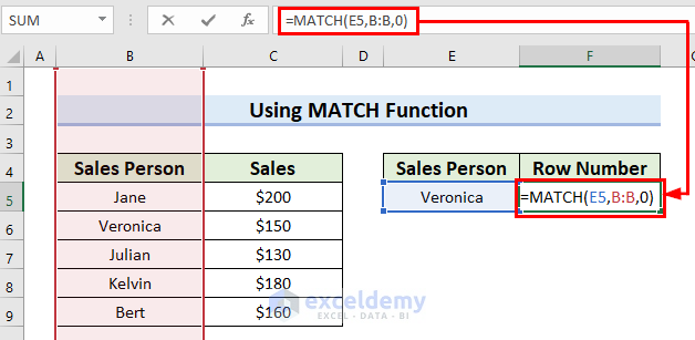
- Press Enter to get the result.
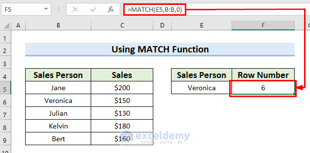
Read More: How to Get Row Number of Current Cell in Excel
Method 2 – Applying IFERROR and MATCH Functions to Return the Row Number in Excel
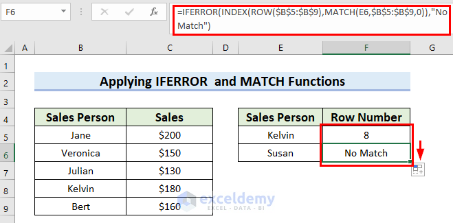
We will find the strings in cells E5 and E6 from the column named Sales Person and return their row numbers in cells F5 and F6.
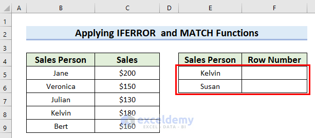
Steps:
- Select the cell where you want to return the row number. We selected cell F5.
- Insert the following formula.
=IFERROR(INDEX(ROW($B$5:$B$9),MATCH(E5,$B$5:$B$9,0)),"No Match")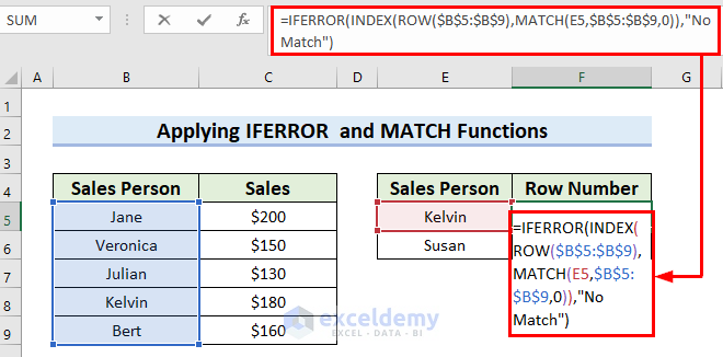
Formula Breakdown
- MATCH(E5,$B$5:$B$9,0) —-> Here, the MATCH function will match the value in cell E5 with cell range B5:B9 for the exact match and return the serial number of the found match.
- Output: 4
- ROW($B$5:$B$9) —-> Here, the ROW function will return the row numbers of cell range B5:B9.
- Output: {5;6;7;8;9}
- INDEX(ROW($B$5:$B$9),MATCH(E5,$B$5:$B$9,0)) —-> turns into
- INDEX({5;6;7;8;9},4) —-> Here, the INDEX function will return the row number that is in serial 4.
- Output: {8}
- INDEX({5;6;7;8;9},4) —-> Here, the INDEX function will return the row number that is in serial 4.
- IFERROR(INDEX(ROW($B$5:$B$9),MATCH(E5,$B$5:$B$9,0)),”No Match”) —-> turns into
- IFERROR(8,”No Match”) —-> Here, the IFERROR function will check for errors, and it will return “No Match” if any error is found.
- Output: {8}
- IFERROR(8,”No Match”) —-> Here, the IFERROR function will check for errors, and it will return “No Match” if any error is found.
- Press Enter.
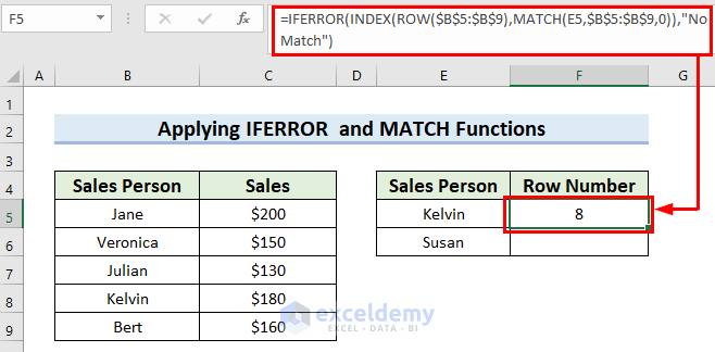
- Drag the Fill Handle down to copy the formula.
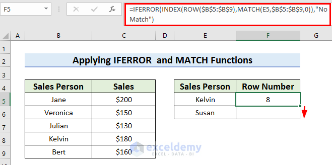
Here’s the result.
Method 3 – Using an Array Formula to Find a String in a Column and Return the Row Number in Excel
We’ll find the string from cell E5 in column and return row number in Excel.
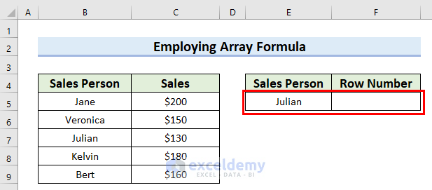
- In cell F5, insert the following formula.
=MAX((B5:B9=E5)*ROW(B5:B9))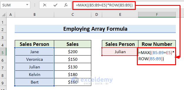
Formula Breakdown
- B5:B9=E5 —-> Here, the formula will check if the value in cell E5 matches the value in cell range B5:B9.
- Output: {FALSE;FALSE;TRUE;FALSE;FALSE}
- ROW(B5:B9) —-> Here, the ROW function will return the row numbers of cell range B5:B9.
- Output: {5;6;7;8;9}
- (B5:B9=E5)*ROW(B5:B9) —-> turns into
- {FALSE;FALSE;TRUE;FALSE;FALSE}*{5;6;7;8;9} —-> Here, the formula will multiply the values.
- Output: {0;0;7;0;0}
- {FALSE;FALSE;TRUE;FALSE;FALSE}*{5;6;7;8;9} —-> Here, the formula will multiply the values.
- MAX((B5:B9=E5)*ROW(B5:B9)) —-> turns into
- MAX({0;0;7;0;0}) —-> Here, the MAX formula will return the highest value found.
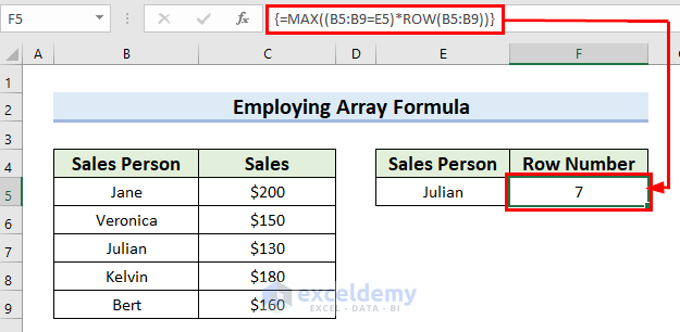
- Output: 7
- MAX({0;0;7;0;0}) —-> Here, the MAX formula will return the highest value found.
- Press Ctrl + Shift + Enter to get the result as it is an array formula. If you are using Office 365 or any updated version of Microsoft Excel, you can press Enter to get the result.
Read More: How to Use Range with Variable Row Number in Excel
Method 4 – Using MATCH and ROW Functions to Find String in Column
We will find the string that is in cell E5 from the column named Sales Person and return the row number in cell F5.
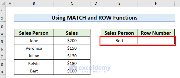
Steps:
- In cell F5, insert the following formula.
=MATCH(E5,B5:B9,0)+ROW(B5:B9)-1 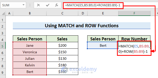
Formula Breakdown
- MATCH(E5,B5:B9,0) —-> Here, the MATCH function will match the value in cell E5 with cell range B5:B9 for an exact match and return the serial number of the found match.
- Output: 5
- ROW(B5:B9) —-> Here, the ROW function will return the row numbers of cell range B5:B9.
- Output: {5;6;7;8;9}
- MATCH(E5,B5:B9,0)+ROW(B5:B9)-1 —-> turns into
- 5+5-1 —-> here, the formula will sum the first two numbers and then subtract 1 from the result.
- Output: 9
- 5+5-1 —-> here, the formula will sum the first two numbers and then subtract 1 from the result.
- Press Enter.
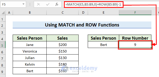
Method 5 – Applying INDEX, MATCH, and ROW Functions in Excel
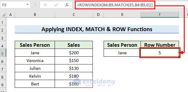
We will find the string in E5 from the column named Sales Person and then return the row number in cell F5.
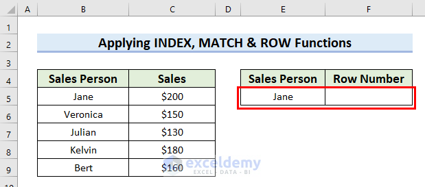
Steps:
- In cell F5, insert the following formula.
=ROW(INDEX(B4:B9,MATCH(E5,B4:B9,0)))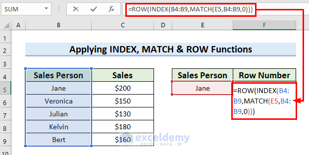
Formula Breakdown
- MATCH(E5,B4:B9,0) —-> Here, the MATCH function will match the value in cell E5 with cell range B5:B9 for the exact match and return the serial number of the found match.
- Output: 2
- INDEX(B4:B9,MATCH(E5,B4:B9,0)) —-> turns into
- INDEX(B4:B9,2) —-> Here, the INDEX function will return the value in serial 2 in cell range B4:B9.
- Output: “Jane”
- INDEX(B4:B9,2) —-> Here, the INDEX function will return the value in serial 2 in cell range B4:B9.
- ROW(INDEX(B4:B9,2)) —-> turns into
- ROW(“Jane”) —-> Here, the ROW function will return the row number of the reference.
- Output: {5}
- ROW(“Jane”) —-> Here, the ROW function will return the row number of the reference.
- Hit Enter.
Method 6 – Use the TEXTJOIN Function to Return Multiple Results
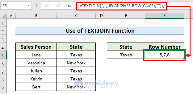
We modified the dataset to contain people’s names and their State. There are more than one Sales Person from the same State. We will find the string in E5 from the column named State and then return their row numbers.
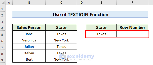
Steps:
- In cell F5, insert the following formula.
=TEXTJOIN(",",,IF(C4:C9=E5,ROW(C4:C9),""))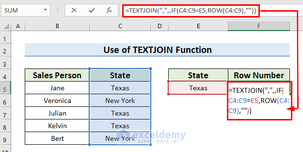
Formula Breakdown
- IF(C4:C9=E5,ROW(C4:C9),””) —-> Here, the IF function will check if the value in E5 matches the value in cell range C4:C9. If it is true then the function will return the row number otherwise it will return blank.
- Output: {“”;5;””;7;8;””}
- TEXTJOIN(“,”,,IF(C4:C9=E5,ROW(C4:C9),””)) —-> turns into
- TEXTJOIN(“,”,,{“”;5;””;7;8;””},””)) —-> Here, the TEXTJOIN function will combine these values from the string.
- Output: “5,7,8”
- TEXTJOIN(“,”,,{“”;5;””;7;8;””},””)) —-> Here, the TEXTJOIN function will combine these values from the string.
- Press Enter if you are using Office 365 or press Ctrl + Shift + Enter.
Method 7 – Using VBA
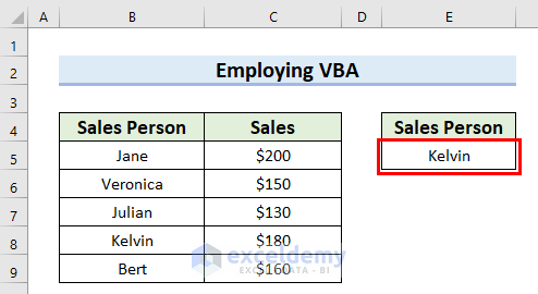
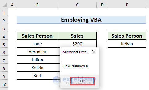
We will find the string in cell E5 from column B and then show the row number in a message box.
Steps:
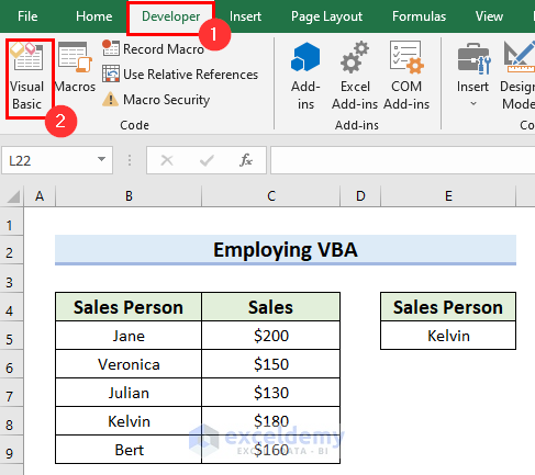
- Go to the Developer tab.
- Select Visual Basic.
The Visual Basic window will open.
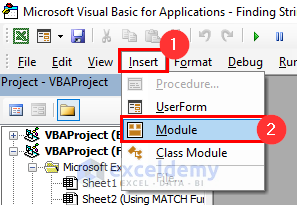
- Select Insert.
- Select Module.
A Module will open.
- Insert the following code.
Sub find_string()
Dim my_WS As Worksheet
Dim string_match As Long
Dim row_number As Long
Dim string_searched As String
Set my_WS = Worksheets("Employing VBA")
string_searched = my_WS.Range("E5").Value
    For row_number = 1 To 100
        If StrComp(my_WS.Range("B" & row_number).Value, string_searched, vbTextCompare) = 0 Then
        string_match = row_number
    Exit For
    End If
    Next row_number
MsgBox "Row Number: " & string_match
End Sub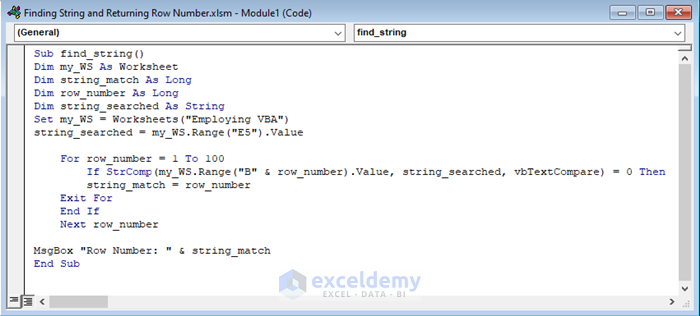
Code Breakdown
- We created a Sub Procedure named find_string().
- We declared a variable named my_WS as Worksheet, a variable named string_match as Long, a variable named row_number as Long, and another variable named string_searched as String.
- We used the Set statement to assign the worksheet named “Employing VBA” as my_WS.
- We set the value in cell E5 as string_searched.
- We used a For Next loop to look through the whole column B.
- We used an IF statement to check if the Value matches any value in column B. Here, in the IF statement, I used the StrComp function to return the value after comparing two strings.
- We used the MsgBox function to show the Row Number in a message box.
- Save the code and go back to your worksheet.
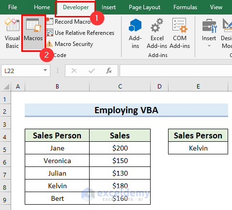
- Go to the Developer tab.
- Select Macros.
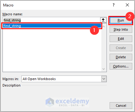
- Select the Sub Procedure you created.
- Select Run.
A MsgBox with the row number of the found string will appear.
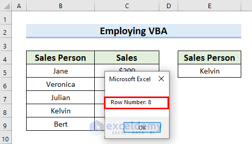
- Select OK to remove the MsgBox.
Practice Section
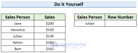
We have provided a practice sheet for you to practice.
Download the Practice Workbook
<< Go Back to Rows in Excel | Learn Excel
Get FREE Advanced Excel Exercises with Solutions!

