What Is Sliding Scale Commission?
Sales employees play a crucial role in any company and motivating them to achieve higher sales targets is essential. Money serves as a powerful motivator in this context. Many companies use sliding scales to determine commissions for their sales teams.
Here’s an example of how sliding scale commissions might work:
- Sales between $0 and $10,000: 10% commission
- Sales between $10,001 and $15,000: 15% commission
- Sales between $15,001 and $35,000: 20% commission
- Sales exceeding $35,000: 25% commission
For instance, if an employee generates sales of less than $10,000, they receive a 10% commission. As sales increase, so does the commission percentage. This approach encourages employees to strive for higher sales targets.
Two Types of Sliding Scales
- Whole Amount Sliding Scale:
- In this type, the employee receives a commission based on the entire sales amount.
- For example, if an employee generates $15,000 in sales, they receive a 15% commission on the entire amount.
- Cumulative Amount Sliding Scale:
- Here, the commission is calculated cumulatively based on different tiers.
- For instance, if an employee generates $15,000 in sales, they receive 10% on the first $10,000 and 15% on the remaining $5,000.
From a company’s perspective, the second type (cumulative amount) is preferred, although the calculation is more complex.
Method 1 – Creating a Sliding Scale Commission Calculator in Excel
- Create a table with three columns: “Name,” “Sales,” and “Commission.”
- Create another table with three columns: “Lowest,” “Highest,” and “Percentage.”
- Enter the total sales amount (e.g., $15,000) in cell E4.
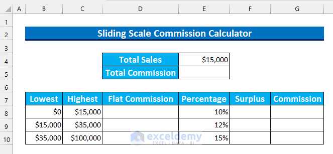
- Calculate Commission Per Tier:
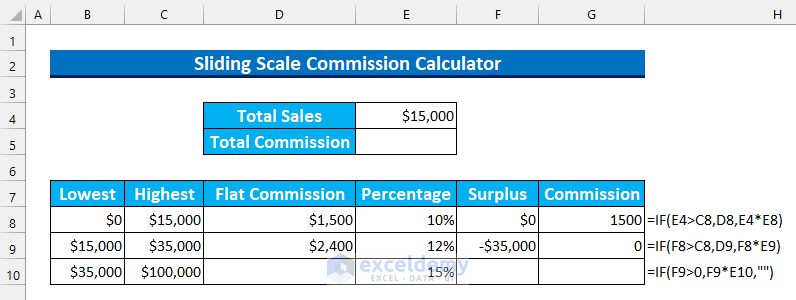
In cell D8, enter the formula:
=C8*E8
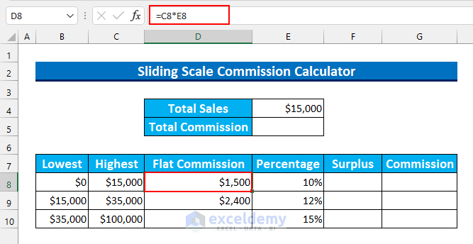
This formula calculates the commission on the sales between $0 and $15,000.
- In cell D9, enter the formula:
=(C9-C8)*E9
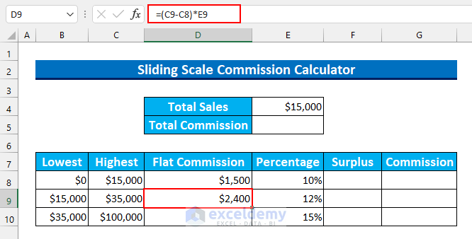
This formula calculates the commission on the remaining amount.
- In cell F8, calculate the surplus amount:
=E4-C8

Here, we calculated the surplus amount by subtracting the Total Sales amount from the highest value of our first sliding scale.
- In cell F9, find the surplus for the second tier:
=F8-C9
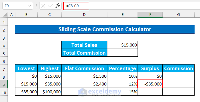
We subtract the previous surplus value from the highest value of the second tier from the sliding commission.
- Commission Breakdown Per Tier – Enter the following formulas:
In Cell G8:
=IF(E4>C8,D8,E4*E8)
This formula checks if Total Sales exceed the first tier, if yes, use the Flat Commission column. As it is exactly the same, it will be10% commission on the Total Sales value.
In Cell G9:
=IF(F8>C8,D9,F8*E9)
If the cell value of F8 is more than cell value C8, it will return the value from cell D9, else the multiplication of cells F8 by E9 will be returned (i.e., compares F8 with C8 and calculates accordingly).
In Cell G10:
=IF(F9>0,F9*E10,"")
If the Surplus value in cell F9 is negative, it will keep the cell blank (i.e., handles negative surplus values).
- The three formulas will look like this.
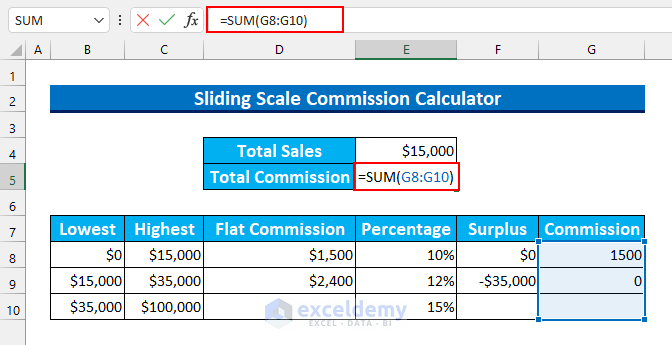
- Total Commission – In cell E5, sum up the commission breakdown values:
=SUM(G8:G10)
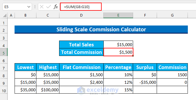
- Press ENTER to calculate the cumulative sliding scale commission.
Method 2 – Using the VLOOKUP Function
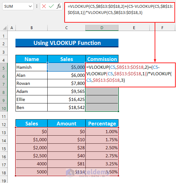
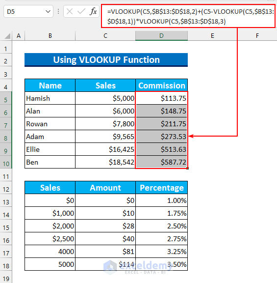
- Select the cell range D5:D10.
- Enter the following formula:
=VLOOKUP(C5,$B$13:$D$18,2)+(C5-VLOOKUP(C5,$B$13:$D$18,1))*VLOOKUP(C5,$B$13:$D$18,3)
Formula Breakdown
-
-
- We use three VLOOKUP functions:
- VLOOKUP(C5,$B$13:$D$18,2)
- Output: 113.75.
- Looks for the value in cell C5 within the B13:D18 range and returns the value from the second column.
- VLOOKUP(C5,$B$13:$D$18,3)
- Output: 0.035.
- Looks for the value in cell C5 within the B13:D18 range and returns the value from the third column.
- C5-VLOOKUP(C5,$B$13:$D$18,1)
- Output: 0.
- Finds the difference between the value in cell C5 and the value from the third column (which is 5000). Since both values are the same, the result is 0.
- The overall formula simplifies to 113.75+0*0.035 =113.75.
-
- Press CTRL+ENTER to Auto-fill the formula for the remaining cells.
Method 3 – SUMPRODUCT and IF Functions
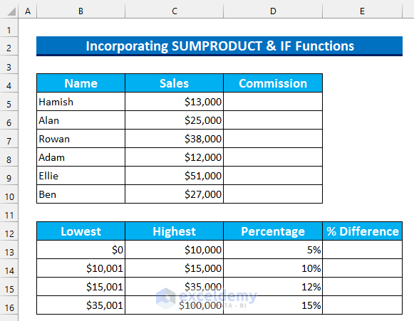
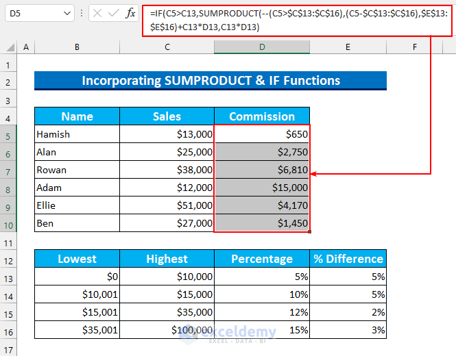
- Select the cell range E14:E16 and enter the formula:
=D14-D13
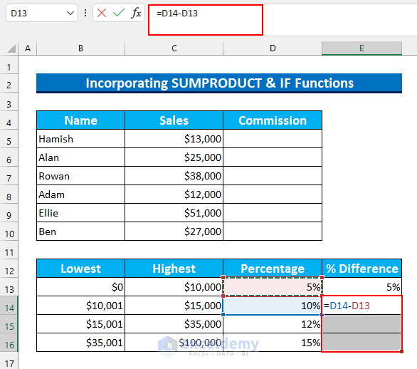
- Press CTRL+ENTER to calculate the percentage difference.
- Formula for Sliding Scale Commission:
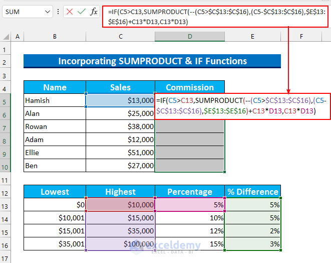
- Select the cell range D5:D10.
- Enter the following formula:
=IF(C5>C13,SUMPRODUCT(--(C5>$C$13:$C$16),(C5-$C$13:$C$16),$E$13:$E$16)+C13*D13,C13*D13)
Formula Breakdown
-
-
- The SUMPRODUCT function combines arrays to calculate the commission.
- The IF function checks if the value from cell C5 exceeds that of cell C13.
- If true, it calculates the commission using the SUMPRODUCT result plus an additional term.
- If false, it uses a simpler calculation based on C13 and D13.
-
- Press CTRL+ENTER to Auto-fill the formula for the remaining cells.
Method 4 – Merging INDEX and MATCH Functions
Sliding Scale Commission on the Whole Amount
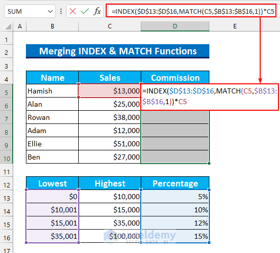
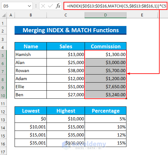
- Select the Cell Range D5:D10.
- Enter the following formula:
=INDEX($D$13:$D$16,MATCH(C5,$B$13:$B$16,1))*C5
Formula Breakdown
-
-
- MATCH(C5,$B$13:$B$16,1)
- This function returns the cell number that matches our criteria.
- We set the criteria to the value from cell C5 (which is $13,000).
- The lookup array is defined as the cell range B13:B16.
- The match type is set to “less than” (typed as 1), resulting in the output of 2.
- The overall formula simplifies to: INDEX($D$13:$D$16,2)*C5 = 1300
- The INDEX function returns the second value from the cell range D13:D16 (which is 0.1).
- We multiply this value by the sales amount to find the sliding commission.
- MATCH(C5,$B$13:$B$16,1)
-
- Press CTRL+ENTER to AutoFill the formula for the remaining cells.
Method 5 – Combining IF and AND Functions
Sliding Scale Commission on the Whole Amount
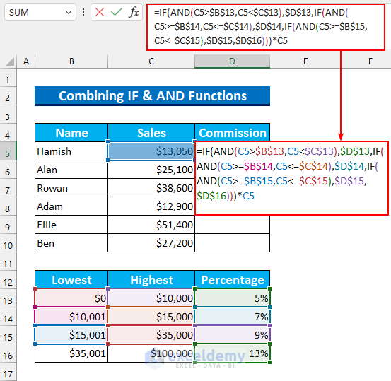
- Enter the following formula in cell D5:
=IF(AND(C5>$B$13,C5<$C$13),$D$13,IF(AND(C5>=$B$14,C5<=$C$14),$D$14,IF(AND(C5>=$B$15,C5<=$C$15),$D$15,$D$16)))*C5
Formula Breakdown
-
-
- We use AND functions inside IF functions in this formula.
- The formula checks where the sales value lies on the sliding scale table.
- It loops through the entire range until it finds the appropriate range.
- The value is then multiplied by the sales figure to determine the sliding commission.
-
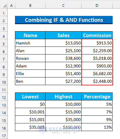
- Press ENTER and use the Fill Handle to autofill the formula.
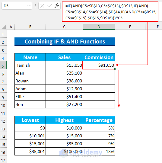
These five formulas demonstrate how to calculate sliding scale commissions in Excel.
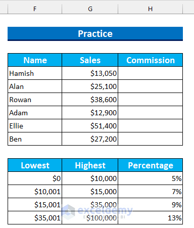
Practice Section
A practice dataset for each method has been included allowing you to practice these methods.
Download the Practice Workbook
You can download the practice workbook from here:
<< Go Back to Commission Bonus | Formula List | Learn Excel
Get FREE Advanced Excel Exercises with Solutions!


I am having a difficult time coming up with the correct calculation and selecting the correct model for a cumulative sliding commission scale. Can you please point me in the right direction. I thought I knew Excel until I ran into this conundrum and realized there is a wealth of capability in Excel for which I have no knowledge. I could merely calculate the individual commission for each transaction but I feel that would be a missed opportunity. Your help is greatly appreciated.
Broker Commission Schedule
Deal Size Range (Low) Deal Size Range (High) “$ Incremental
Commission” “% Incremental
Commission” “Cumulative
Commission” Rate delta “Effective
Commission”
$0 $5,000,000 $250,000 5.00% $250,000 0.00% 5.00%
$5,000,001 $10,000,000 $150,000 3.00% $400,000 2.00% 4.00%
$10,000,001 $15,000,000 $75,000 1.50% $475,000 1.50% 3.17%
$15,000,001 $30,000,000 $150,000 1.00% $625,000 0.50% 2.08%
$30,000,001 $45,000,000 $112,500 0.75% $737,500 0.25% 1.64%
$45,000,001 $60,000,000 $75,000 0.50% $812,500 0.25% 1.35%
$60,000,001 $100,000,000 $200,000 0.50% $1,012,500 0.00% 1.01%
$100,000,001 $150,000,000 $250,000 0.50% $1,262,500 0.00% 0.84%
$150,000,001 $200,000,000 $250,000 0.50% $1,512,500 0.00% 0.88%
$200,000,001 $250,000,000 $250,000 0.50% $1,762,500 0.00% 0.81%
$250,000,001 $300,000,000 $250,000 0.50% $2,012,500 0.00% 0.75%
$300,000,001 $350,000,000 $250,000 0.50% $2,262,500 0.00% 0.72%
$350,000,001 $400,000,000 $250,000 0.50% $2,512,500 0.00% 0.69%
$400,000,001 $450,000,000 $250,000 0.50% $2,762,500 0.00% 0.67%
$450,000,001 $500,000,000 $250,000 0.50% $3,012,500 0.00% 0.65%
$500,000,001 $550,000,000 $190,000 0.38% $3,202,500 0.12% 0.63%
$550,000,001 $600,000,000 $190,000 0.38% $3,392,500 0.00% 0.61%
$600,000,001 $650,000,000 $190,000 0.38% $3,582,500 0.00% 0.59%
$650,000,001 $700,000,000 $190,000 0.38% $3,772,500 0.00% 0.57%
$700,000,001 $750,000,000 $190,000 0.38% $3,962,500 0.00% 0.56%
$750,000,001 $800,000,000 $125,000 0.25% $4,087,500 0.13% 0.54%
$800,000,001 $850,000,000 $125,000 0.25% $4,212,500 0.00% 0.52%
$850,000,001 $900,000,000 $125,000 0.25% $4,337,500 0.00% 0.51%
$900,000,001 $950,000,000 $125,000 0.25% $4,462,500 0.00% 0.49%
Thank you, JOHN SCURAS, for your comment.
You can use the below formula to determine your commission of the model.
=IF(H36>C33,SUMPRODUCT(–(H36>$C$33:$C$56),(H36-$C$33:$C$56),$D$33:$D$56)+C33*E33,C33*E33)
Here, H36 is the sales amount, C33 is your first Deal Size Range (High), C33:C56 is all values for Deal Size Range (High) column, D33:D56 is all values from the % incremental commission column, and E33 is the first value of the incremental commission (5%).
Best Regards,
Bishwajit
Team ExcelDemy