In this article, we will use an Excel formula to find the last row number with data for two cases – either when the last row is blank or when it is non-blank. The output of the last row number with data will not be the same in both cases, so we will use different approaches.
Scenario 1 – Using an Excel Formula to Find Non-Blank Last Row Number with Data
Method 1.1 – Using a Formula with ROW and ROWS Functions
The ROW function in Excel returns the row number from the active worksheet.
The ROWS function in Excel returns the number of rows in a specified reference.
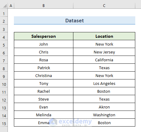
We will find the last row number of the following dataset in cell E5.
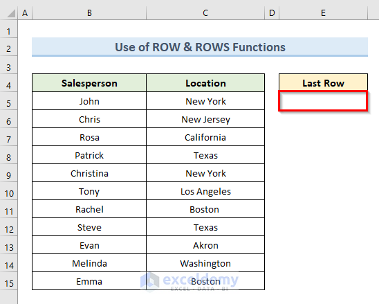
STEPS:
- Select cell E5.
- Insert the following formula in that cell:
=ROW(B5:C15) + ROWS(B5:C15)-1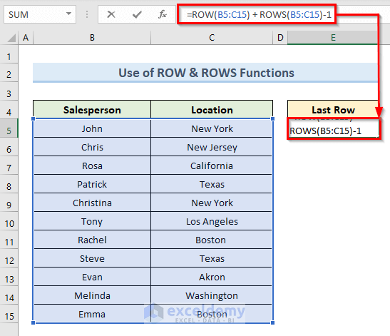
- Press Enter.
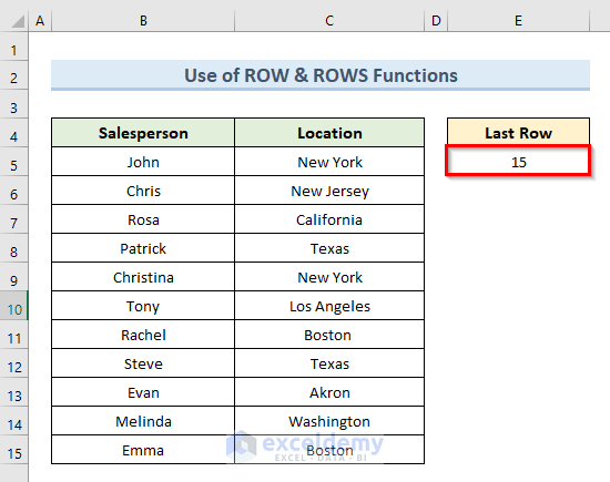
- The above action returns the row number of the last row from the data range in cell E5. We can see that the number of the last row is 15.
Read More: How to Find Last Row with a Specific Value in Excel
Method 1.2 – Using a Formula combining MIN, ROW, and ROWS Functions
The MIN function in Excel returns the data’s smallest number value from a data range.
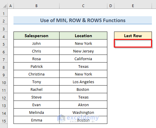
STEPS:
- Select cell C5.
- Insert the following formula in that cell:
=MIN(ROW(B5:C15))+ROWS(B5:C15)-1- Press Enter.
- The above command returns the number of the last row in cell E5.
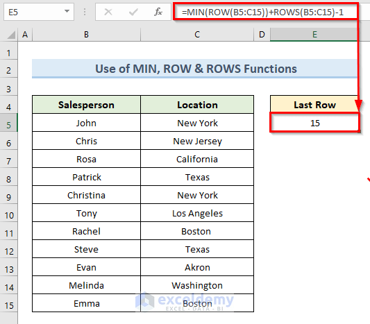
How Does the Formula Work?
- ROW(B5:C15))+ROWS(B5:C15)-1: This part returns the array of row numbers from the last row, which is row number 15.
- MIN(ROW(B5:C15))+ROWS(B5:C15)-1: Returns the minimum row number in cell E5 which is row number 15.
Method 1.3 – Using a Formula combining ROW, INDEX, and ROWS Functions
In Microsoft Excel, the INDEX function returns the value at a certain position in a range or array.
We will find the number of the last row from the following dataset.
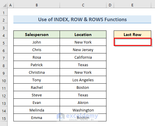
STEPS:
- Select cell E5.
- Input the following formula in that cell:
=ROW(INDEX(B5:C15,1,1))+ROWS(B5:C15)-1- Press Enter.
- We get the last row number of our data range in cell E5 which is 15.
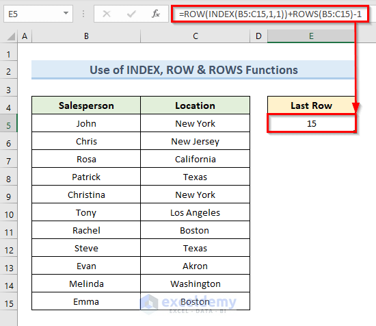
How Does the Formula Work?
- INDEX(B5:C15,1,1): This part creates an array of the data range (B5:C15).
- ROWS(B5:C15)-1: This part subtracts 1 from the total row numbers.
- ROW(INDEX(B5:C15,1,1))+ROWS(B5:C15)-1: Returns the minimum row number in cell E5 which is row number 15.
Scenario 2 – Finding Both Blank and Non-Blank Last Row Number with Data in Excel
Method 2.1. Inserting the MAX Formula to Find the Last Row of Data in Excel
The Excel MAX function provides the greatest value in a specified set of data.
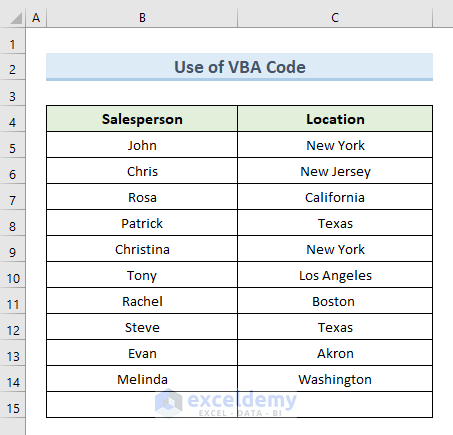
We see that the last row of the following dataset doesn’t contain any value.
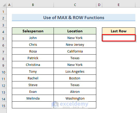
Let’s see the steps to do this method.
STEPS:
- Select cell E5.
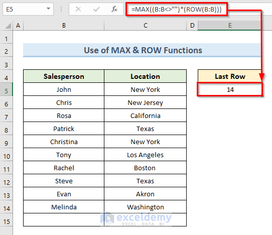
- Input the following formula in that cell:
=MAX((B:B<>"")*(ROW(B:B)))- Press Enter.
- We get the last row number in cell E5 which is 14. It excludes the last row of our data range which is blank.
Read More: How to Find Last Non Blank Cell in Row in Excel
Method 2.2 – Combining MATCH and REPT Functions to Find the Last Row of Data in Excel
The MATCH function in Excel searches a range of cells for a specified item and then returns the item’s relative location in the range.
The REPT function in Excel repeats specific text a given number of times. We can use the REPT function to fill a cell with multiple instances of a text string.
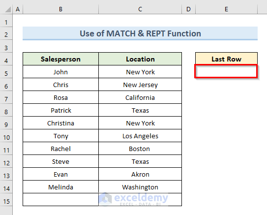
STEPS:
- Select cell E5.
- Insert the following formula in that cell:
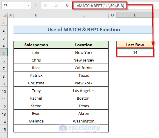
=MATCH(REPT("z",50),B:B)- Press Enter.
- In cell E5 we get the number of the last row with data in our dataset.
How Does the Formula Work?
- REPT(“z”,50): This part repeats the text ‘z’ 50 times.
- MATCH(REPT(“z”,50),B:B): In this part, the MATCH function looks in column B for our 50-character text string of ‘z’. The formula returns the location of the last non-blank cell since it cannot find it.
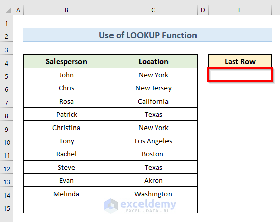
Method 2.3 – Using the Excel LOOKUP Formula to Find the Last Row of Data in Excel
The LOOKUP function belongs to the Excel Lookup and Reference functions. The LOOKUP function returns the comparable value from another one-row or one-column range after performing an approximate match lookup.
STEPS:
- Select cell E5.
- Enter the following formula in that cell:
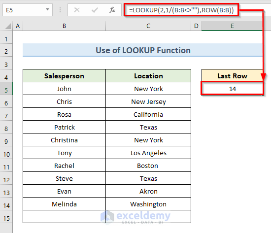
=LOOKUP(2,1/(B:B<>""),ROW(B:B))- Press Enter.
- We can see the last row number of our data range in cell E5 which is 14.
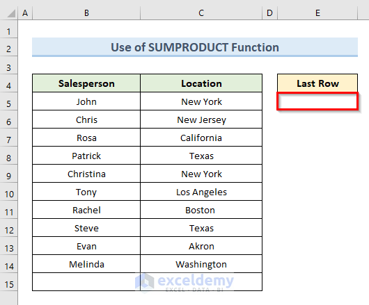
Method 2.4 – Using SUMPRODUCT Function to Find the Last Row of Data in Excel
The SUMPRODUCT function in Excel returns the sum of matching ranges or arrays’ products.
STEPS:
- Select cell E5.
- Enter the following formula in that cell:
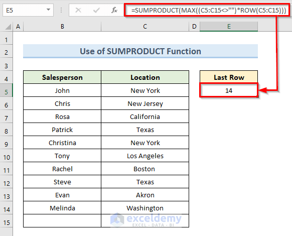
=SUMPRODUCT(MAX((C5:C15<>"")*ROW(C5:C15)))- Press Enter if you are using ‘Microsoft Office 365’. Otherwise you have to press Ctrl + Shift + Enter to run an array.
- We get the last row number with data in cell E5.
How Does the Formula Work?
- ROW(C5:C15): This part returns the row number for each cell in range (C5:C15).
- MAX((C5:C15<>””): This part returns the highest number from the array of row numbers.
- SUMPRODUCT(MAX((C5:C15<>””)*ROW(C5:C15))): The SUMPRODUCT function is used to calculate the above two arrays and return a value in the selected cell.
Method 2.5 – Using VBA code to Find the Last Row with Data in Excel
STEPS:
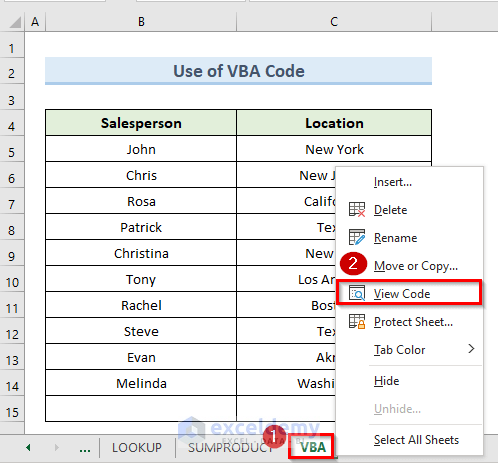
- Right-click on the sheet name of the active sheet.
- Click on the option ‘View Code’.
- A new blank VBA module will appear.
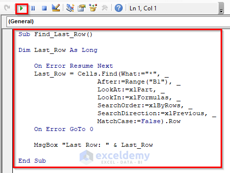
- Enter the following code in the blank module:
Sub Find_Last_Row()
Dim Last_Row As Long
    On Error Resume Next
    Last_Row = Cells.Find(What:="*", After:=Range("B1"), _
                    LookAt:=xlPart, LookIn:=xlFormulas, _
                    SearchOrder:=xlByRows, SearchDirection:=xlPrevious, _
                    MatchCase:=False).Row
    On Error GoTo 0
    MsgBox "Last Row: " & Last_Row
End Sub- Click on Run or press F5 to run the code.
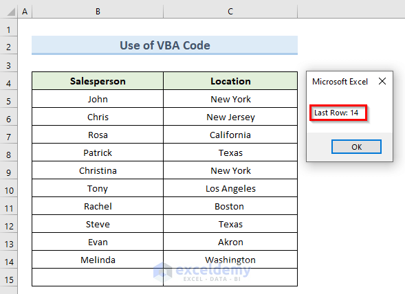
- The message box that appears shows that the last row number with data is 14.
Download Practice Workbook
You can download the practice workbook from here.
Related Articles
- How to Find Last Cell with Value in Column in Excel
- Excel Find Last Column With Data
- How to Find Highest Value in Excel Column
- How to Find Lowest Value in an Excel Column
- How to Find Last Cell with Value in a Row in Excel
<< Go Back to Find Value in Range | Excel Range | Learn Excel
Get FREE Advanced Excel Exercises with Solutions!
