Example 1 – Excel Formula with MOD and ROW Functions to Insert Rows between Data
We will use the combination of the MOD and ROW functions to insert rows between data. Suppose we have the below dataset containing several people’s names and ages. We will insert blank rows after every 3 rows in this dataset. Follow the below steps to perform the task.
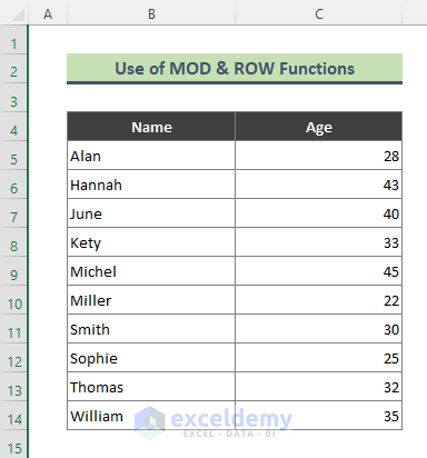
Steps:
- Add a helper column to the parent dataset and use the below formula in Cell D5.
=MOD(ROW(D5)-ROW($D$4)-1,3)- Press Enter.
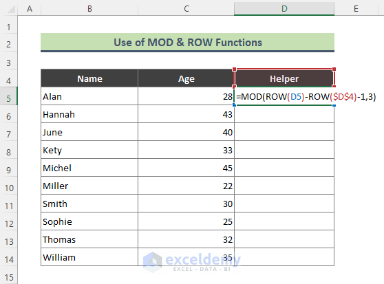
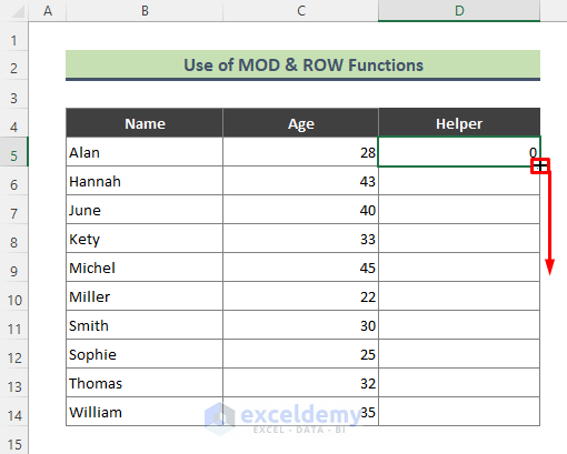
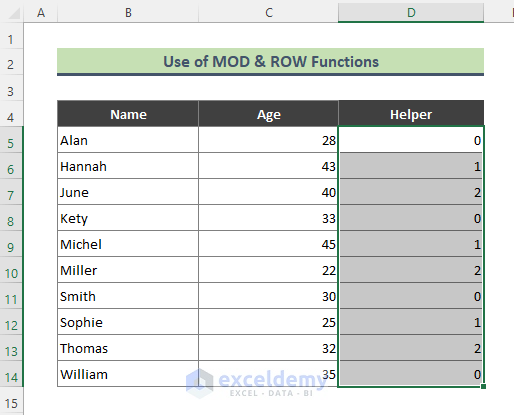
- Use the Fill Handle (+) tool to copy the formula to the rest of the cells.
- Select the helper column and press Ctrl + F to bring the Find and Replace dialog box.
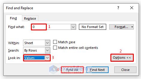
- In the Find and Replace dialog, enter zero (0) in the Find what box, click on Options, choose Values from the Look in drop-down, and click on Find All.
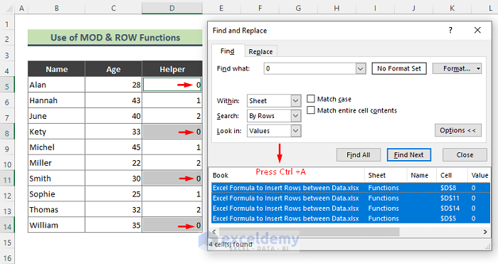
- Excel will return the references of cells in the helper column that contains zero. Press Ctrl + A to select all of them.
- Those cells will be selected in the dataset, too. Close the Find and Replace dialog.
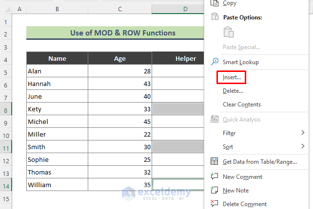
- Among all of the selected cells containing 0, unselect only the first one. Right-click on any of the selected cells and click on Insert.
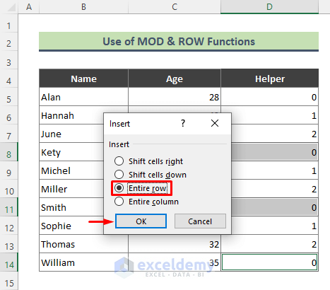
- The Insert dialog will appear.
- Click on the Entire Row option and press OK.
- We can see blank rows are added after every three rows.
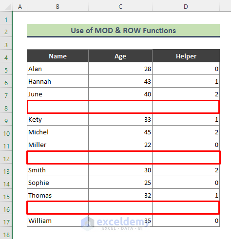
How Does the Formula Work?
- ROW(D5)
Here the ROW function returns the row number of Cell D5 which is:
{5}
- ROW($D$4)
Now, the ROW function returns the row number of Cell D4:
{4}
- MOD(ROW(D5)-ROW($D$4)-1,3)
Lastly, the MOD function returns the remainder when 0 is divided by 3. Here 3 is the value of N. If you want to insert blank rows between every 4 rows, N will be 4. The result is:
{0}
Read More: How to Insert Multiple Blank Rows in Excel
Method 2 – Add Blank Rows between Data Using Helper Column in Excel
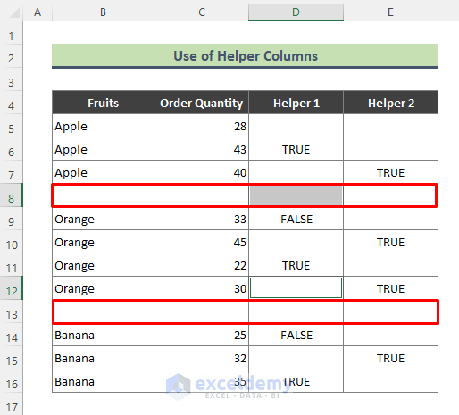
Suppose we have a dataset containing fruit names and their order quantities. There are three types of fruits in the dataset and similar types of fruits are written in sequences. But at first glance, you cannot tell immediately at what rows a fruit’s name is changed. If you insert a blank row between the changing data, it will be easier to separate each fruit type.
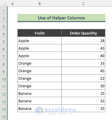
Steps:
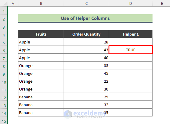
- Insert a helper column to the parent dataset and use the below formula in Cell D6.
=B6=B5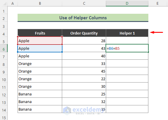
- Hit Enter.
- Add another Helper column to the dataset and use the following formula in Cell E7.
=B7=B6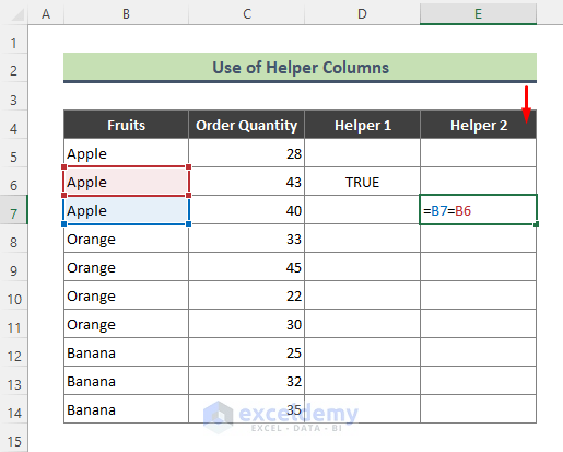
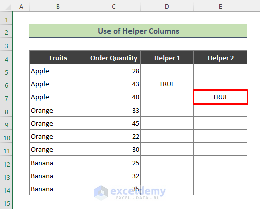
- We will get the following result.
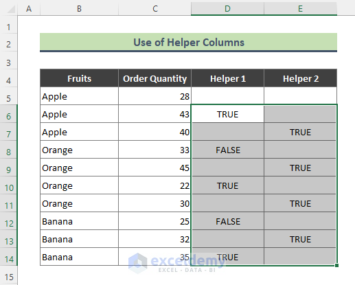
- Select D6:E7 and drag the Fill Handle down.
- Select both Helper 1 and Helper 2 columns and press Ctrl + F to get the Find and Replace dialog.
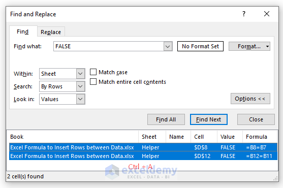
- Type FALSE in the Find what box, choose Values from the Look in drop-down menu, and click on Find All.
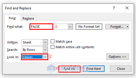
- We will get the cell that contains FALSE. Use Ctrl + A to select all the results and close the Find and Replace dialog.
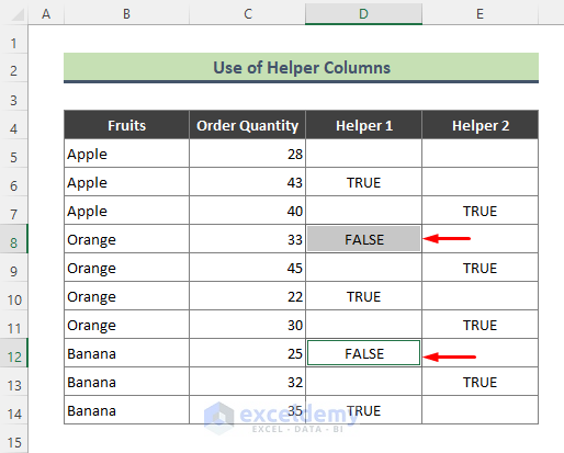
- As have selected all the cells that contain FALSE, those cells will be selected in the main dataset, too.
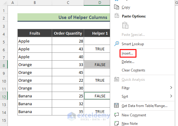
- Right-click on the selection and select Insert.
- When the Insert dialog comes up, click on the Entire Row and press OK.
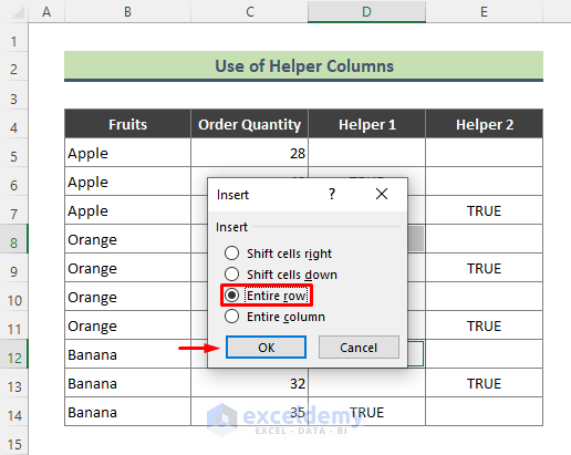
- We can see a blank row is added whenever the fruit names change.
Read More: Insert Multiple Rows After Every Other Row in Excel
Download the Practice Workbook
Related Articles
- Shortcuts to Insert New Row in Excel
- How to Insert Multiple Rows in Excel
- How to Insert Rows in Excel Automatically
- Cannot Insert Row in Excel
- Excel Fix: Insert Row Option Greyed Out in Excel
- How to Insert Row Below in Excel
<< Go Back to Insert Rows | Rows in Excel | Learn Excel
Get FREE Advanced Excel Exercises with Solutions!

