How to Hide a Formula but Allow Input in Excel – 2 Methods

This is an overview:

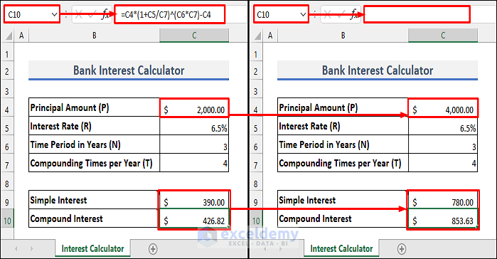
Consider the following bank interest calculator:

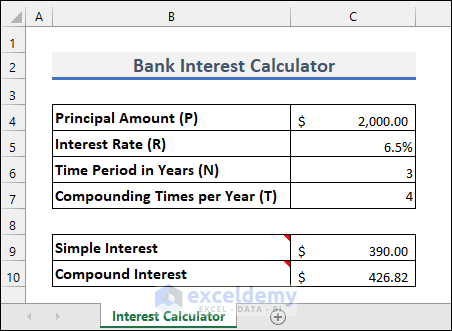
You want to allow users to input data in C4:C7, but you don’t want to allow them to change the formulas in C9:C10.

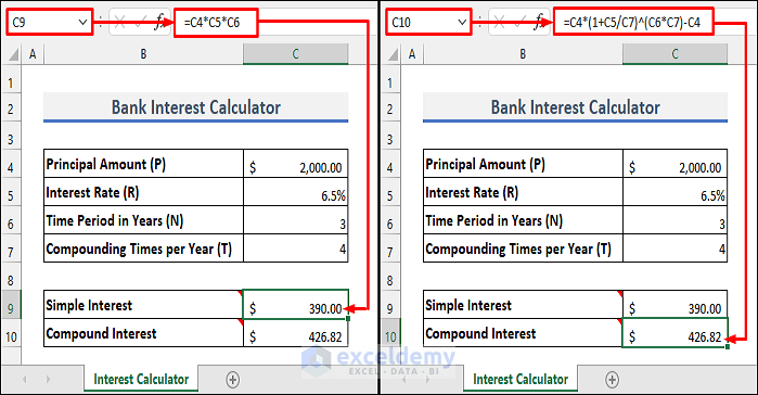
Method 1 – Protecting the Excel Worksheet to Hide the Formula but Allow Input

Steps

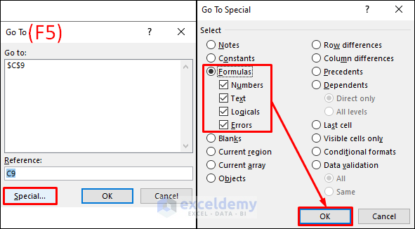
• Select C4:C10. You can also select all the formulas in the Excel sheet using the Go To Special command: Press F5 >> Special >> Formulas >> OK.

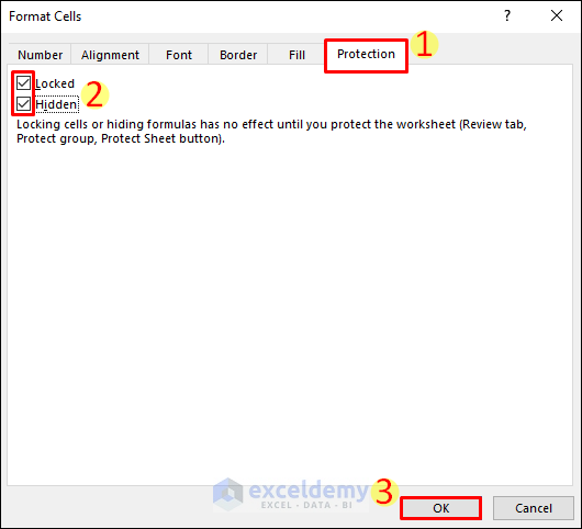
• Press CTRL+1 to open the Format Cells dialog box.
• Check Locked and Hidden.
• Click OK.

• Select the cells you want to keep editable. Here, C4:C7.
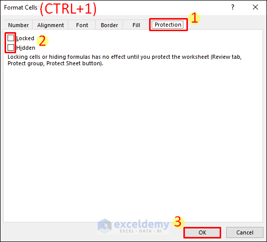
• Press CTRL+1 and go to the Protection tab.
• Keep Locked and Hidden unchecked.
• Click OK.

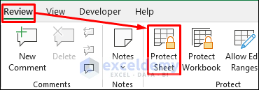
• Select Protect Sheet in the Review tab.

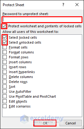
• Enter a password (optional).
• Check Select locked cells and Select unlocked cells.
• Click OK.

If you select the cells containing formulas, you won’t see the formula in the formula box.

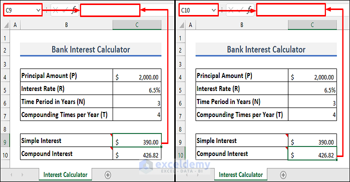
If you try to edit those cells, you will see the following error.

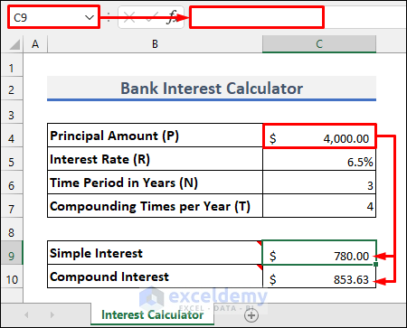
But you can input values in C4:C7, and the results in C9:C10 will be updated.

Read More: How to Hide Formulas from Other Users in Excel

Method 2 – Using a VBA Macro to Hide the Formula but Allow Input

• Press ALT+F11 to open the Microsoft VBA window.
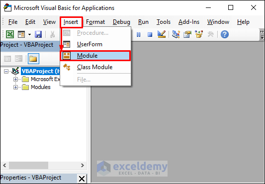
• Select Insert >> New Module.

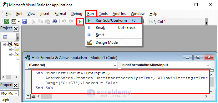
• Copy the following code:

Sub HideFormulaButAllowInput()

ActiveSheet.Protect Userinterfaceonly:=True, AllowFiltering:=True

Range("C4:C7").Locked = False

End Sub

• Paste the code in the blank module.
• Press F5 to run the code.

Download Practice Workbook

Download the practice workbook.

Related Articles

• How to Hide Formula in Excel without Protecting Sheet
• Hide Formulas and Display Values in Excel
• How to Hide Formulas in Excel Until Data Is Entered

<< Go Back to Hide Excel Formulas | Excel Formulas | Learn Excel