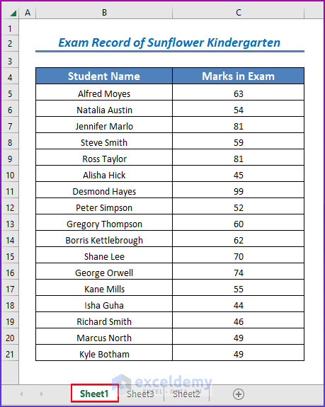
We have a worksheet called Sheet1 with the names of some students and their marks. We will add hyperlinks to this sheet in another worksheet of the same workbook or a different workbook.
Method 1 – Inserting the HYPERLINK Function to Add a Hyperlink to Another Sheet in Excel
Case 1.1 – Adding a Hyperlink to Different Worksheets in the Same Workbook
We have opened a worksheet called Sheet2 in the same workbook and created an empty table there to insert the hyperlinks for the marks.
Steps:
- Select a cell and enter the HYPERLINK function.
The Syntax of the HYPERLINK Function is:
=HYPERLINK(link_location,friendly_name)To create a link to cell C5 of Sheet1, the link_location will be #Sheet1!C4. The friendly_name argument is the displayed text. We’ll use Marks.
- Use the following complete formula:
=HYPERLINK("#Sheet1!C5","Marks")- Press Enter.
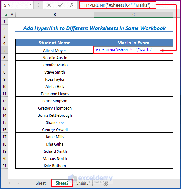
- Use the Fill Handle tool and drag it down from the C5 to C21.
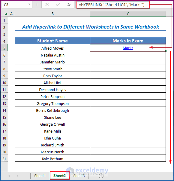
- You will get all the hyperlinked marks in the below image.
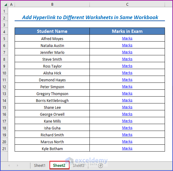
- The symbol (#) denotes that the worksheet is from the same workbook.
Read More: Excel Hyperlink to Another Sheet Based on Cell Value
Case 1.2 – Adding Hyperlinks to Different Worksheets in Different Workbooks
To create a hyperlink to a worksheet of a different workbook, enter the name of the workbook before the worksheet name, enclosed by a square bracket [ ], inside the HYPERLINK function.
Steps:
- To create a hyperlink to cell C5 of Sheet1 of Book1, the HYPERLINK formula will be:
=HYPERLINK("[Book1]Sheet1!C5","Marks")- You will get the same results for the different worksheets.
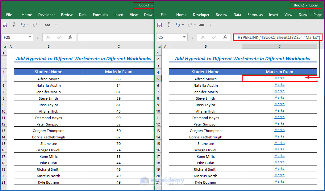
- The two workbooks must be in the same folder. Otherwise, you have to enter the full location (file path) of the workbook.
Read More: How to Hyperlink to Cell in Excel
Method 2 – Using the Context Menu to Add a Hyperlink to Another Sheet in Excel
Case 2.1 – Adding a Hyperlink to Different Worksheets in the Same Workbook
Steps:
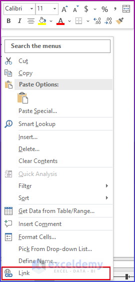
- Right-click on the cell where you want to enter the hyperlink.
- Select Link from the options.
- You will get a dialog box called Insert Hyperlink.
- Select Place in this Document from the left panel.
- In the Text to Display box, enter the name of the link to show. We put Marks.
- In the Type the Cell reference box, enter the cell reference of the cell that you want to link: C5.
- In the select a place in this document box, select the worksheet name to which you want to link: Sheet1.
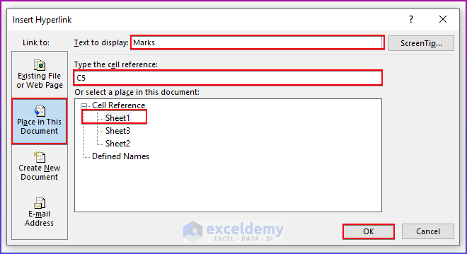
- Click OK.
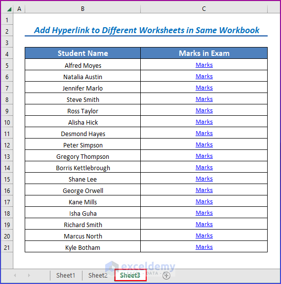
- You can AutoFill the links to the other cells.
Read More: Excel Hyperlink with Shortcut Key
Case 2.2 – Adding Hyperlink to Different Worksheets in Different Workbooks
Steps:
- Follow the same procedure as discussed above to open the Insert Hyperlink dialog box.
- Choose Existing File or Web Page.
- Find the workbook to which you want to link. We want to link to Book1.
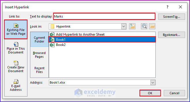
- Click OK. You will find a hyperlink created on your selected cell connecting you to the desired workbook.
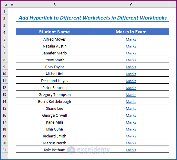
- You can’t link to a specific cell in a different workbook in this way. You can just link to the workbook.
Read More: Excel Hyperlink to Cell in Another Sheet with VLOOKUP
Download the Practice Workbook
Excel Hyperlink to Another Sheet: Knowledge Hub
- Excel Hyperlink to Another Sheet Based on Cell Value
- Create a Drop Down List Hyperlink to Another Sheet
- Create Button to Link to Another Sheet
- Excel Hyperlink to Cell in Another Sheet with VLOOKUP
<< Go Back To Hyperlink in Excel | Linking in Excel | Learn Excel
Get FREE Advanced Excel Exercises with Solutions!


doesn’t work in Excel360 (online version)
Hello Leonardo Lagos,
You can use the HYPERLINK function in Excel 360 online version.
Insert the following formula in your formula bar: =HYPERLINK(“#’SheetName’!A1”, “Link Text”)
But unfortunately, you can’t directly use the context menu to add a hyperlink to another sheet in Excel Online. You’ll need to use the formula approach described above.
Regards
ExcelDemy