How to create a Hyperlink to a Cell in Another Sheet with VLOOKUP Function – 3 Steps

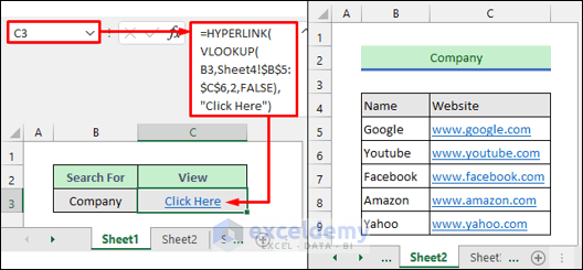
This is an overview:

The Excel HYPERLINK Function

Function Objective:

The HYPERLINK function in Excel creates a shortcut or link that opens a document on a hard drive, a network server, or on the Internet.

Syntax:

HYPERLINK(link_location, [friendly_name])

Arguments:

• link_location : Required. Asks for the link address or its location.
• friendly_name : Optional. Displays this name for the created link.

The Excel VLOOKUP Function

Function Objective:

The VLOOKUP function in Excel looks for a value in the leftmost column of a table and returns a value in the same row from a specified column.

Syntax:

VLOOKUP(lookup_value, tabble_array, col_index_num, [range_lookup])

Arguments:

• lookp_value : Required. Searches for this value within a range.
• tabble_array : Required. The range to search for the lookup_value.
• col_index_num : Required. The column number in the table_array to return a value matching the lookup_value.
• [range_lookup] : Optional. 0 or FALSE by default mean Exact Match. 1 or TRUE mean Approximate Match.

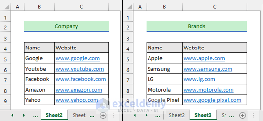
The following dataset is in Sheet2 and Sheet3.

Sheet2 contains the list of top companies in the USA. Sheet3 contains the list of top smartphone brands.

Step 1 – Create a Helper Sheet

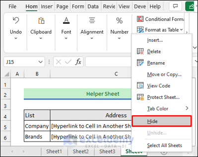
• Create a helper sheet containing keywords and their location. Here, Sheet4. Notice that the hash (#) sign can replace the name of This Workbook.

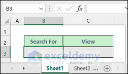
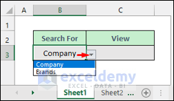
To search for keywords and generate hyperlinks in Sheet1, create a drop-down list with the keywords:

• Select B3.

Step 2 – Apply Data Validation

• Press ALT+D+L+L or select Data >> Data Validation to open the Data Validation window.
• Choose List in Allow: (Settings tab).
• Enter the following formula in Source:.
• Click OK.

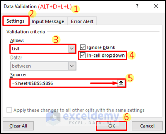
The drop-down list is displayed.

• Choose a keyword.

Read More: How to Add Hyperlink to Another Sheet in Excel

Step 3 – Enter the HYPERLINK-VLOOKUP Formula

• Enter the following formula in C3.

It will create a clickable link. The VLOOKUP function returns the link_location argument for the HYPERLINK function.

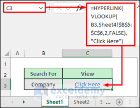
• If you remove the friendly_name argument, you will be able to see the address of the link.

• Hide the helper sheet.

Read More: Excel Hyperlink to Another Sheet Based on Cell Value

If the VLOOKUP Hyperlink Cannot Open a Specified File

The addresses of the keywords contain the sheet names and cell references only:

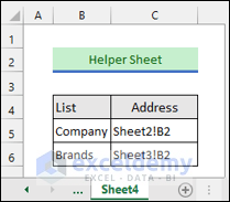
• Excel will display “Cannot open the specified file.”

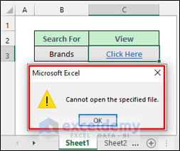
• Add a hash (#) sign or the workbook name inside third brackets before the addresses. You can also use the formula below:

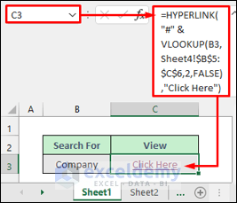
Read More: Hyperlink in Excel Not Working

Create a Hyperlink to a Sheet in a Different Excel Workbook

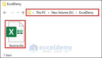
You have a different source workbook in the following path:

• It contains the following dataset.

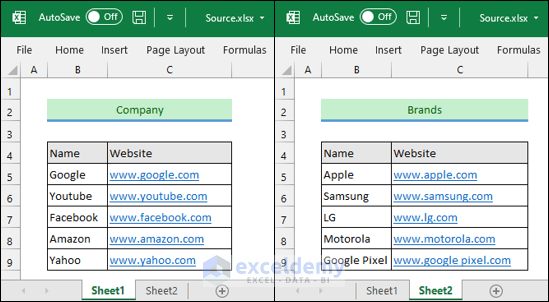
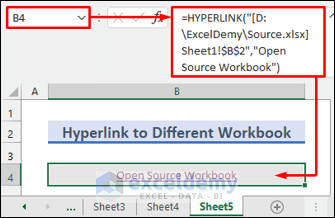
To create a hyperlink to go to the source workbook from the active workbook.

• Enter the following formula in B4.

• Click the hyperlink to go to the source workbook (you need to manually change the file path whenever you change the location of the source file).

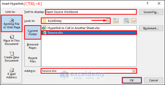
• You can also press CTRL+K while in B4 and use the Insert Hyperlink window.

Read More: How to Create a Drop Down List Hyperlink to Another Sheet in Excel

Things to Remember

• Use the Edit Links feature in the Data tab to modify links.

Download Practice Workbook

Download the practice workbook.

Related Articles

• How to Hyperlink to Cell in Same Sheet in Excel
• How to Combine Text and Hyperlink in Excel Cell
• How to Edit Hyperlink in Excel
• How to Create Dynamic Hyperlink in Excel
• How to Copy Hyperlink in Excel
• How to Convert Text to Hyperlink in Excel
• How to Create Button to Link to Another Sheet in Excel

<< Go Back To Excel Hyperlink to Another Sheet | Hyperlink in Excel | Linking in Excel | Learn Excel