Consider the following dataset of products and their IDs. We can search for a specific product using a predetermined value or a given value in a cell.
Excel If Cell Begins with Certain Text, Then Return Value: 3 Examples
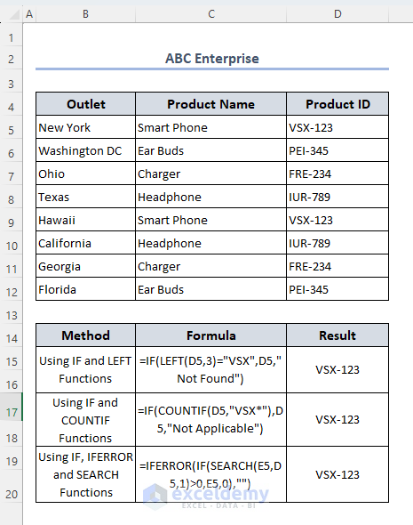
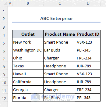
The dataset below represents the Outlets of ABC Enterprise with Product Name, and Product ID stored in every outlet. Some products are common in different outlets so the Product ID will also be common. We want to find out if the cell begins with a certain text and then returns value using this dataset.
Method 1. Combination of IF and LEFT Functions
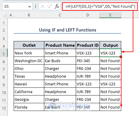
- Select cell E5 and enter the following formula:
=IF(LEFT(D5,3)="VSX",D5,"Not Found")
- Drag the Fill Handle icon.
Formula Breakdown
LEFT(D5,3)
the LEFT function extracts 3 letters or characters from the left or start of cell D5.
Result: VSX
IF(LEFT(D5,3)=”VSX”,D5,”Not Found”)
The IF function compares the result of the LEFT function and returns the value if true or shows Not Found if false.
Result: VSX-123
Note:
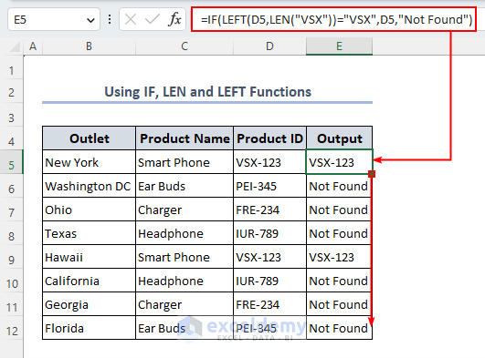
If you don’t want to write down the length of the search term in the formula manually, you can use the LEN function like the below formula. This option is the alternative to make the formula dynamic.
=IF(LEFT(D5,LEN(“VSX”))=”VSX”,D5,”Not Found”)
Method 2 – Using IF and COUNTIF Functions
- Select cell D5 and apply the following formula there.
=IF(COUNTIF(D5,"VSX*"),D5,"Not Applicable")
- Drag down the Fill Handle to apply the same formula in the entire dataset.
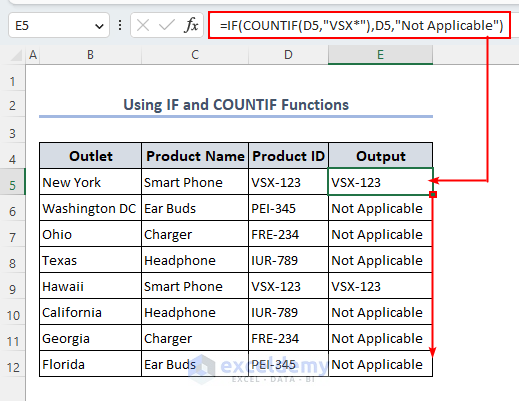
A Wildcard (*) is used in the end of the required word. That means this word is in the beginning of the string.
Formula Breakdown
COUNTIF(D5,”VSX*”)
This function determines if there’s text starting with VSX or not in cell D5. If found, it returns 1. Otherwise, it returns 0.
Result: 1
IF(COUNTIF(D5,”VSX*”), D5,”Not Applicable”)
Here, the IF function shows the final output. If the output of the COUNTIF function is 1 then the final output shows as the data of D5 otherwise “Not Applicable”.
Result: VSX-123
Method 3 – Combination of IF, IFERROR, and SEARCH Functions
- Select cell F5 and apply the following formula.
=IFERROR(IF(SEARCH(E5,D5,1)=1,E5,0),"")
- Drag down the fill handle or double-click on the fill handle to copy it through the column.
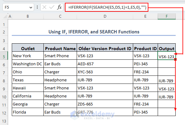
Formula Breakdown
SEARCH(E5,D5,1)
The SEARCH function is used to search similar data from cell D5 to cell E5. 3rd argument indicates search word must be located at the start of cell D5.
Result: 1
IF(SEARCH(E5,D5,1)=1,E5,0)
Here, the IF function shows the final output. If the output of the SEARCH function fulfills the condition then the final output shows as the data of D5 otherwise “Not Applicable”.
Result: VSX-123
IFERROR(IF(SEARCH(E5,D5,1)=1,E5,0),””)
The IFERROR function is to avoid errors in results. Here, for any error formula will show a blank cell otherwise result in the IF function.
Result: VSX-123
Note:
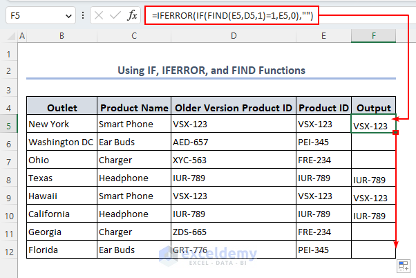
When we need matching with case-sensitivity, use this formula:
=IFERROR(IF(FIND(E5,D5,1)=1,E5,0),"")
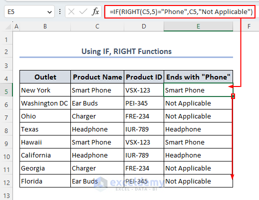
If a Cell Ends with Certain Text, then Return Value in Excel
- Select cell E5 to apply the formula:
=IF(RIGHT(C5,5)="Phone",C5,"Not Applicable")
- Drag down the fill handle to execute this process.
How to Check If a Cell Contains Certain Text in Excel
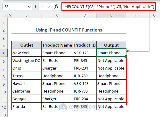
- Use the wildcard (*) while applying the formula in cell E5.
=IF(COUNTIF(C5,"*Phone*"),C5,"Not Applicable")
- Once you use the wildcard it will find out that particular text from anywhere in the string.
How to Check If a Cell Starts with a Number in Excel
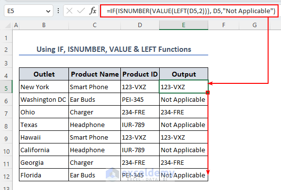
- We have used the following formula on cell E5 and dragged the Fill Handle icon.
=IF(ISNUMBER(VALUE(LEFT(D5,2))), D5,"Not Applicable")
Formula Breakdown
LEFT(D5,3)
LEFT function shows the first 3 letters from the beginning as the output.
Result:
VALUE(LEFT(D5,3))
Here, this function shows the value of the 3 characters from the beginning as we used the LEFT function.
Result: 123
ISNUMBER(VALUE(LEFT(D5,3)))
This function identifies if the function matches the conditions. Here, the ISNUMBER function verifies if the output of the VALUE function matches the condition. If the condition matches the output will be TRUE.
Result: True
IF(ISNUMBER(VALUE(LEFT(D5,2))), D5,”Not Applicable”)
Lastly, if the condition matches then the IF function shows the final output. Here the final output is the value of D5 otherwise the output shows “Not Applicable”
Result: 123-VXZ
How to Count If a Cell Begins with a Specific Text in Excel
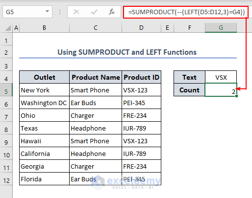
We will count the cells that start with a certain text or data using the combination of LEFT and SUMPRODUCT functions.
- Set the desired text on cell G4.
- Select cell G5 to apply the formula there.
=SUMPRODUCT(--(LEFT(D5:D12,3)=G4))
Formula Breakdown
LEFT(D5:D12,3)
The LEFT function shows the 3 values from the beginning of the total dataset here as the range is D5:D12.
Result: [VSX, PEI, FRE, IUR, VSX, IUR, FRE, PEI]
SUMPRODUCT(–(LEFT(D5:D12,3)=G4))
The SUMPRODUCT function shows the number of match data. Here, the lookup value is VSX from cell G4.
Result: 2
Things to Remember
- The FIND function is case-sensitive so if you use the FIND function make sure the formula matches the case with the lookup value.
- While using the SUMPRODUCT function we use (–). This double unary controls which values should be included in the formula. It makes the formula more powerful.
Download the Practice Workbook
<< Go Back to Text | If Cell Contains | Formula List | Learn Excel
Get FREE Advanced Excel Exercises with Solutions!

