Excel If Cell Color Is Green Then Show or Customize Outputs

You can find people asking online for formulas to work with using the IF function, where they want to use a specific cell color as the condition. Until the latest version of Excel, it is not directly possible. But still, there is some work around that. And with a little help from the Excel macros, you can easily perform such tasks. In this tutorial, we are going to see the extent of what you can do with cell value if the cell color is green or any other specific color in Microsoft Excel.

Things You Can Do If Cell Color Is Green (or Any Other Color) in Excel

Before going through the kinds of stuff you can do if the cell color is green or any other color, you have to define a custom function with the help of name defining feature in Excel. No matter the operation you want to perform you need to do this beforehand. But if you have done it once and do multiple of the task listed below, creating the function once will be enough.

1. If Cell Color Is Green Then Set Cell Value

In the first section, we are going to set cell values if the cell color is green in this Excel dataset. From the dataset, we can see that our second and fifth entries are green. We want to associate “Absent” with them and associate “Present” with the rest.

Follow these steps to see how you can create the custom function in Excel and then set the cell value if the cell color is green or any other color.

Steps to Define Custom Function:

• First of all, go to the Formulas tab on your ribbon.
• Then select Name Manager from the Defined Names

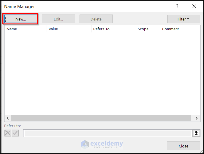
• As a result, the Name Manager box will open up. Now click on New on top of the box.

• After that, in the New Name box, write down a name for the function in the Name field, and in the Refers to field, write down the following.

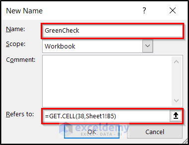
• Finally, click on OK. Now you will have the formula ready called GreenCheck that can be used for other purposes.

Steps to Set Values:

• If you want to find out the color code of the green or any other color you are having, just select cell C5 and write down the following formula.

• Then press Enter and click and drag the fill handle to the end to find values for all.

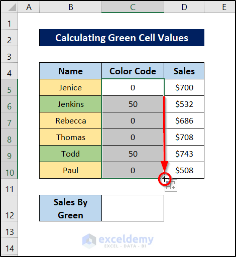
So we can see the color code of the type of green in our dataset is 50. You can clear these values now.

• To get the desired values in our cells, select cell C5 now and write down the following formula.

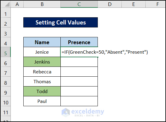
• Then press Enter.

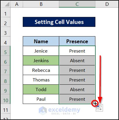
• After that, select the cell again. Now click and drag the fill handle icon to the end of the list to replicate the formula for the rest of the cells.

This way, we can set different values if the cell color is green or any other color.

2. If Cell Color Is Green Then Modify Cell Value

Let’s say there are values already associated with the cells. If you want to modify these values now, this section is can be helpful for you. Here are the steps you can follow to modify cell values in a dataset.

Steps to Define Custom Function:

• First of all, go to the Formulas tab on your ribbon.
• Then select Name Manager.

• As a result, the Name Manager box will open up. Now click on New on top of the box.

• After that, in the New Name box, write down a name for the function in the Name field, and in the Refers to field, write down the following.

• Finally, click on OK. Now you will have the formula ready called GreenCheck that can be used for other purposes.

Steps to Modify Cell Values:

• Now let’s make a chart similar to the one in the previous section. For that, select cell C5 and write down the following formula.

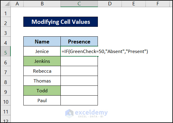
• Then press Enter.

• After that, select the cell again. Now click and drag the fill handle icon to the end of the list to replicate the formula for the rest of the cells.

• Now to modify these values, let’s say, we want the third entry to be green too. For that, select cell B6 and go to the Home tab of your ribbon.
• Then select Format Painter from the Clipboard group.

• Now click on cell B7.

The value of cell C7 will now automatically change to “Absent”.

3. If Cell Color Is Green Then Remove Cell Value

Now let’s say there are values already set on the dataset and you want to remove the values based on color. This section will show you how to remove cell values if the cell color is green from an Excel spreadsheet. But first, you need the custom function.

Steps to Define Custom Function:

• First of all, go to the Formulas tab on your ribbon.
• Then select Name Manager from the Defined Names

• As a result, the Name Manager box will open up. Now click on New on top of the box.

• After that, in the New Name box, write down a name for the function in the Name field, and in the Refers to field, write down the following.

• Finally, click on OK. Now you will have the formula ready called GreenCheck that can be used for other purposes.

Steps to Remove Cell Values:

Let’s say the dataset has values shown below.

To remove the values associated with the green cells follow these steps.

• First, select cell C5 and write down the formula.

• Then press Enter.

You may not see any changes yet depending on your dataset.

• Now select cell C5 again and click and drag the fill handle icon to the end to replicate the formula.

You can see from the figure that the cell values have been removed from the Excel spreadsheet if the cell color of the adjacent cell is green.

4. If Cell Color Is Green Then Count Cells

In this section, we are going to count cells of specific colors. We are choosing green for the demonstration. Let’s say the dataset is like this.

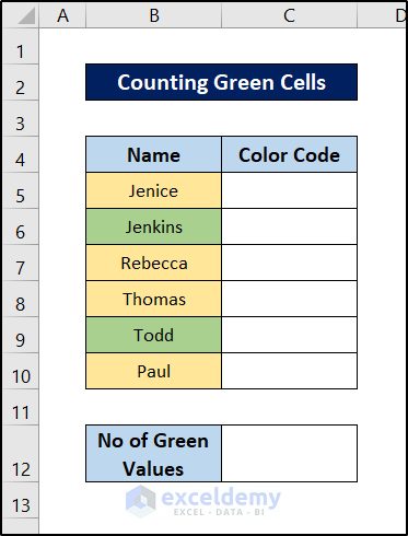
To count the number of cells filled with green or any color we need the help of the COUNTIF function. But first, we need to define the custom function.

Steps to Define Custom Function:

• First of all, go to the Formulas tab on your ribbon.
• Then select Name Manager from the Defined Names

• As a result, the Name Manager box will open up. Now click on New on top of the box.

• After that, in the New Name box, write down a name for the function in the Name field, and in the Refers to field, write down the following.

• Finally, click on OK. Now you will have the formula ready called GreenCheck that can be used for other purposes.

Steps to Count Cells:

• To count the green cells now, select cell C5 and write down the following formula.

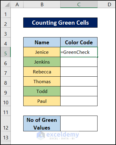
• Then press Enter.

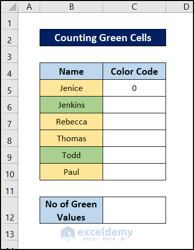
• After that, select the cell again. Then click and drag the fill handle icon to the end of the column to fill the cells with the formula.

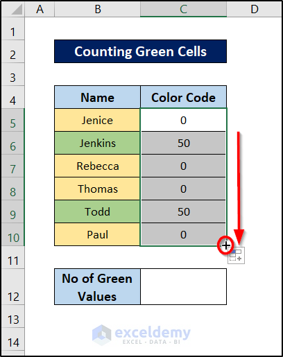
Now we have all the color codes of the adjacent cells in the dataset.

• Next, select cell C12 to enter the count of green cells.

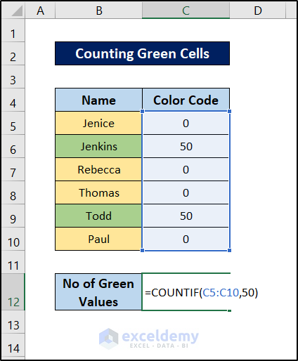
• Finally, press Enter.

This way you can count cells in Excel if the cell color is green or any other specific color.

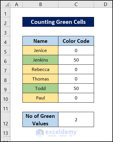
5. If Cell Color Is Green Then Sum Cell Values

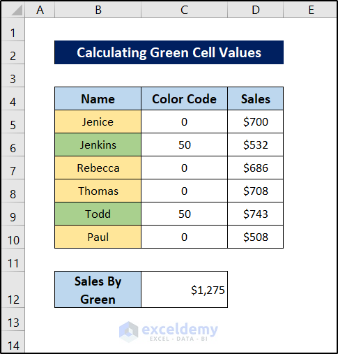
Now let’s assume there are other values associated with the rows of the color-coded cells. For example, let’s look at the following dataset.

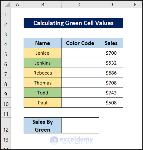
The way these color code functions are set up, the color code column has to be on the right of the colored cells. Nevertheless, we need the help of the SUMIF function for this task.

Follow these steps to see how you can create the custom function and then find the sum of the values associated with green cells.

Steps to Define Custom Function:

• First of all, go to the Formulas tab on your ribbon.
• Then select Name Manager from the Defined Names

• As a result, the Name Manager box will open up. Now click on New on top of the box.

• After that, in the New Name box, write down a name for the function in the Name field, and in the Refers to field, write down the following.

• Finally, click on OK. Now you will have the formula ready called GreenCheck that can be used for other purposes.

Steps to Sum Cell Values:

• First, select cell C5 and write down the following formula.

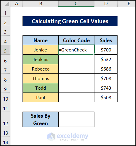
• Then press Enter.

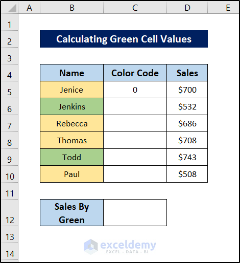
• After that, select the cell again and click and drag the fill handle icon to the end of the list to replicate the formula.

• Next, select cell C12 and write down the formula.

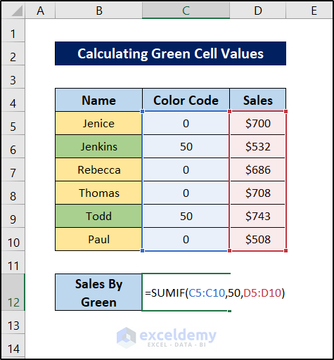
• Finally, press Enter.

This way you can calculate the sum of cell values if the adjacent cell is green or any other color.

Download Practice Workbook

You can download the workbook used for the demonstration from the link below.

Conclusion

This concludes the different operations we can perform if the cell color is different like green in Excel. Hopefully, you have grasped the idea of working with different cell colors and using custom functions to accomplish tasks in Microsoft Excel. I hope you found this guide helpful and informative. If you have any questions or suggestions, let us know in the comments below.

Related Articles

• Excel Color Index Formula
• If Cell Color Is Red Then Execute Different Functions in Excel
• VBA to Check If Font Color is Red Then Return Results in Excel

<< Go Back to Excel Get Cell Color | Excel Cell Format | Learn Excel