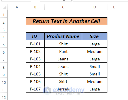
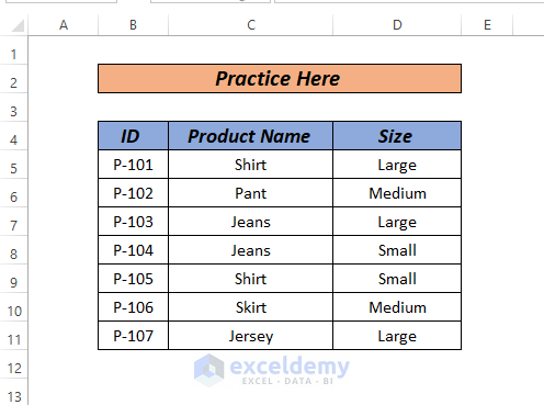
To explain detecting and adding text to cells, let’s use a sample dataset containing ID, Product Name, and Size.
Method 1 – If Cell Contains Text Then Add Text in Another Cell Using ISTEXT Function
Steps:
- Type the following formula in cell E5:
=IF(ISTEXT(C5), "Correct", "Incorrect")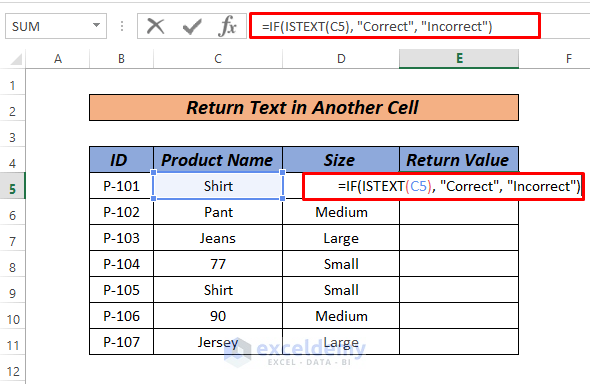
- Press the Enter key.
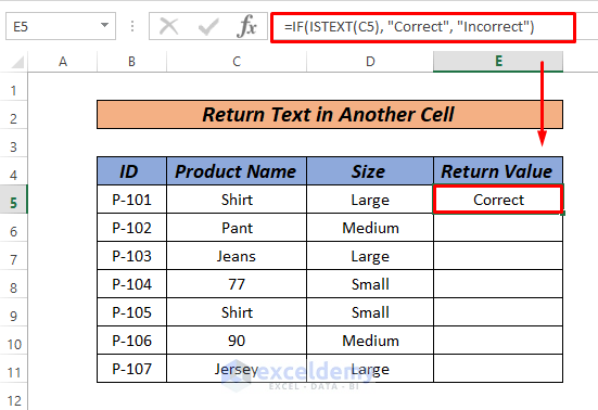
- Drag down the fill handle to AutoFill the rest of the series.
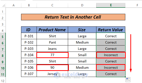
ISTEXT(reference) checks whether the referenced cell has a text-only value, then the IF function returns “Correct” or “Incorrect” based on the result of the check.
Method 2 – If Cell Contains Specific Text Then Add Text in Another Cell Using IF Function
Suppose you want to look for a text value “shirt” in the Product Name column.
Steps:
- Type the following formula in cell E5:
=IF(C5="Shirt", "Yes", "")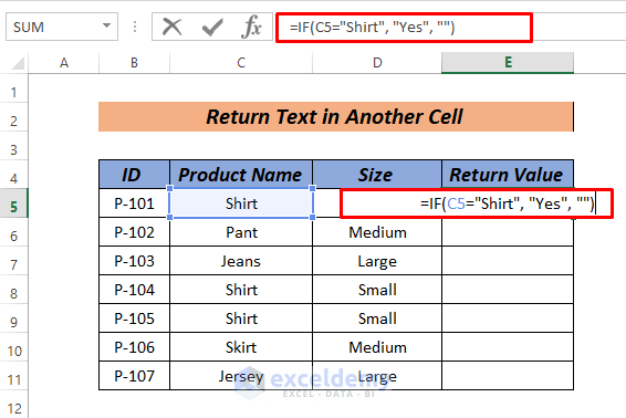
- Press Enter.
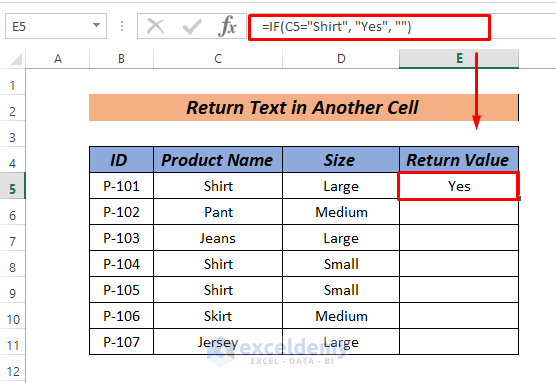
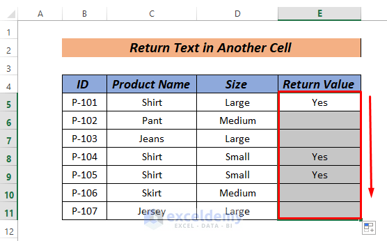
You will get Yes as a return value every time a cell contains Shirt as a text value or a blank cell otherwise.
- Drag down the fill handle to see the result in the rest of the cells.
Method 3 – Using Search Along with ISNUMBER Function
Steps:
- Type the following formula in cell E5:
=IF(ISNUMBER(C5), "", "Text")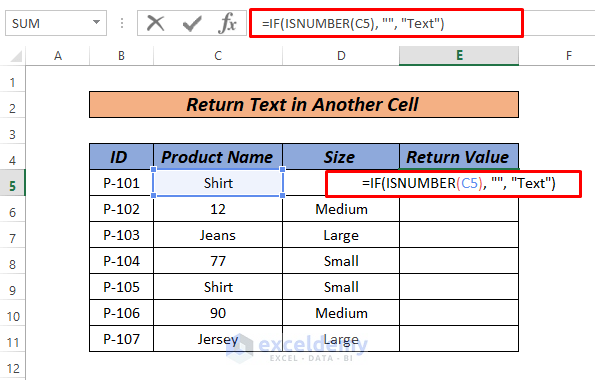
- Hit Enter to apply.
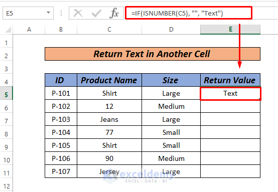
- Drag down the fill handle to AutoFill the rest of the series.
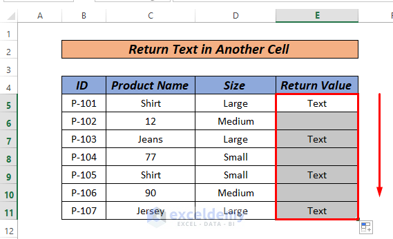
ISNUMBER returns the value as TRUE or FALSE depending on whether the cell contains only a number. Using the IF function we’re telling Excel to return the TRUE as a blank cell and FALSE as Text.
Method 4 – If Cell Contains Many Texts then Add Text in Another Cell Using Combined Formula
Steps:
- Type the following formula in cell E5:
=IF(AND(ISNUMBER(SEARCH("Shirt",C5)), ISNUMBER(SEARCH("Black",C5))), "Yes","")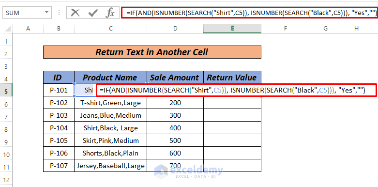
- Press the Enter key.
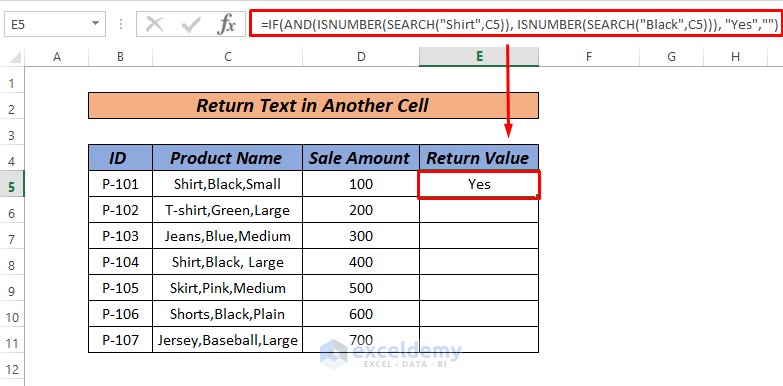
- Drag down the fill handle to the other cells in the E column.
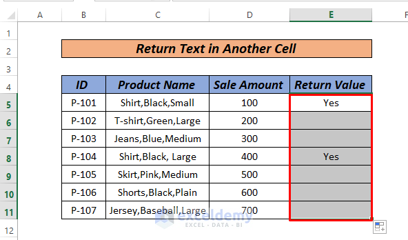
For the example, ISNUMBER(SEARCH(“Shirt”,C5)) gives the output TRUE, ISNUMBER(SEARCH(“Black”,C5) also gives TRUE as output. AND function will count the value as TRUE or If both the output is TRUE otherwise False. The SEARCH function returns the value as a number.
Method 5 – Using VLOOKUP Function to Add Text in Another Cell
Let’s look for a specific value in our Product Name containing text, and then return the Size associated with it.
Steps:
- First, type the following formula in cell E5.
=VLOOKUP(F6,C5:D11,2,FALSE)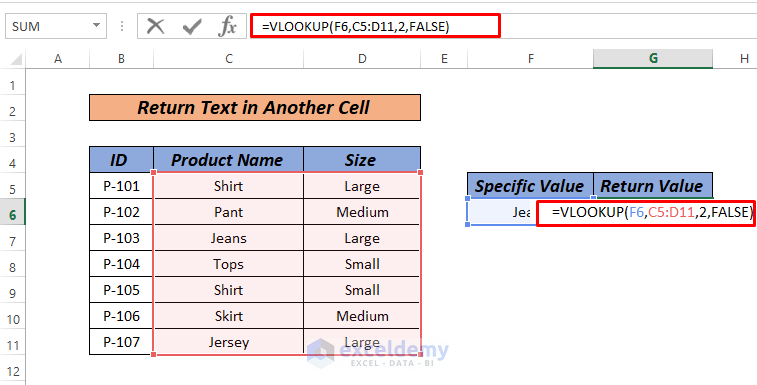
- Press the Enter key.

With VLOOKUP, we are looking for the text Jeans (in cell F6) in the data range C5:D11 and want the return value from the Size column which is associated with it, which is why we used 2 as the column index number.
Method 6 – IF with COUNTIF Function to Add Text If Cell Contains Text
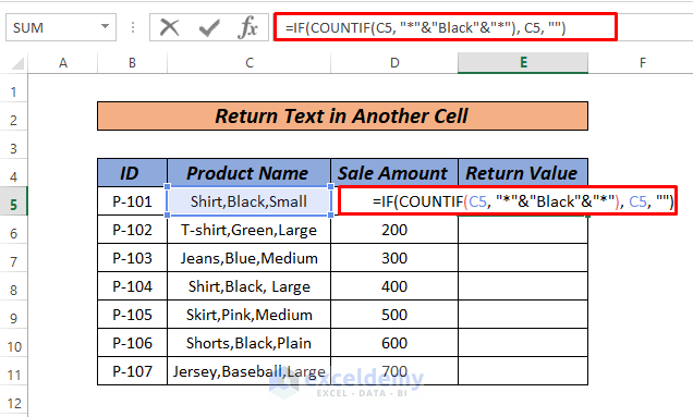
Let’s look for cells that have Black as a text in them and want to return the full text in another column.
Steps:
- Type the following formula in cell E5:
- Press the Enter key.
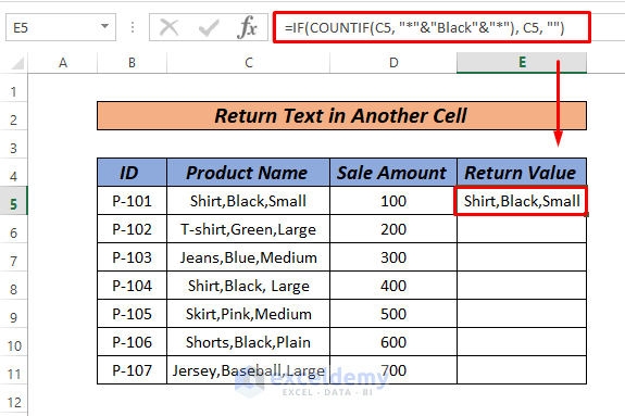
- Drag down the fill handle to AutoFill the rest of the cells.
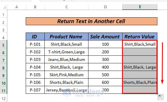
COUNTIF(C5, “*”&”Black”&”*”) will return the value 1 if Black text exist in cell C5. Then =IF(1, C5, “”) will give output as it is in C5 which is Shirt, Black, Small.
Practice Section
We’ve attached a practice workbook where you may practice these methods.
Download Practice Workbook
<< Go Back to Text | If Cell Contains | Formula List | Learn Excel
Get FREE Advanced Excel Exercises with Solutions!


WE have 20 people in our leagues each season.
I would like to have the list alphabetize automatically their names each time sheet is opened.
Once we assign everyone a number in column E,
have G5 look for all players assigned 1 and print in the format i have shown in H5, I5
and continue until all 10 teams show the team member names
Player Number First Name Last Name Number Assigned Team Number
1 Adera Quick 4 1 Joe Slow & Barb Pine
2 Al Knol 6
3 Barb Tamp 9 2 Nate Late & Bob Stout
4 Barb Pine 1
5 Bob Henry 10 3
6 Bob Stout 2
7 Bryan Smith 3 4
8 Cindy Dime 5
9 Dave Radclif 6 5
10 George Plum 8
11 Jane Tilson 10 6
12 Joe Slow 1
13 Ken Gibson 7 7
14 Mack Long 3
15 Nate Late 2 8
16 Ned Brow 5
17 Ray Erskine 9 9
18 Shelly Early 8
19 Steve Ready 4 10
20 Sue Baxter 7
Hello Kenneth,
To auto sort the list alphabetize based on their names you can use the SORT function.
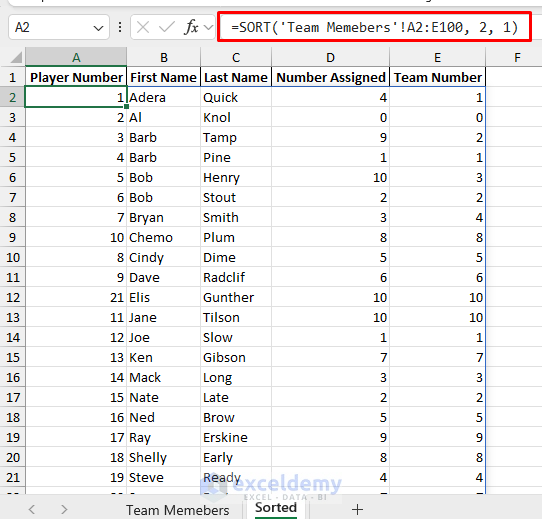
Here, I used the SORT function to sort your data automatically each time you enter new player name.
=SORT(‘Team Memebers’!A2:E100, 2, 1)
To make a team used the TEXTJOIN and FILTER function.
=TEXTJOIN(“, “, TRUE, FILTER($A$2:$A$21, $E$2:$E$21=H1))
If you are comfortable with VBA then you also can use the code instead of SORT function.
Insert the code in the Team Members sheet.
Download the Excel File:
Auto Sort Team Members Name and Assign Team
Regards
ExcelDemy