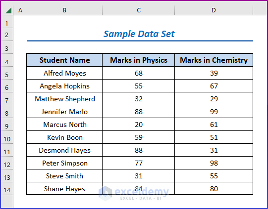
Here we’ve got a data set with the Names of some students and their Marks in Physics and Chemistry.
Method 1 – Combining IF and OR Functions in Excel for OR Type Criteria Between Multiple Ranges
Let’s fail a student if they score lower than 40 in a single subject. Here’s how you can use OR for that.
Steps:
- Select the E5 cell and enter this formula:
=IF(OR(C5<40,D5<40),"Fail","Pass")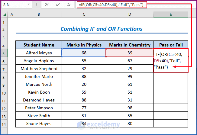
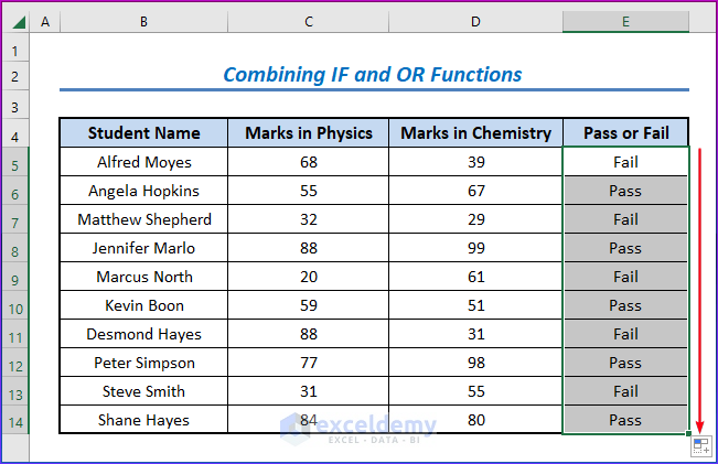
- Drag the Fill Handle to copy this formula to the rest of the cells.
- You can see the students who have failed in at least one subject have been judged as Fail.
- C4<40 returns TRUE if the mark in cell C4 (Mark in Physics) is less than 40, and returns FALSE otherwise. Same goes for D4<40.
- OR(C4<40,D4<40) returns TRUE if at least one cell between C4 and D4 contains a value lower than 40.
- Finally, IF(OR(C4<40,D4<40),”Fail”,”Pass”) returns “Fail” if it encounters a TRUE. Otherwise returns “Pass”.
Read More: How to Use Excel IF Function with Range of Values
Method 2 – Nesting IF and AND Functions in Excel for AND Type Criteria Between Multiple Ranges
Let’s reformulate the same pass criteria as before to be that a student passes if both of their scores are above 40.
Steps:
- Choose the E5 cell and enter this formula:
=IF(AND(C5>=40,D5>=40),"Pass","Fail")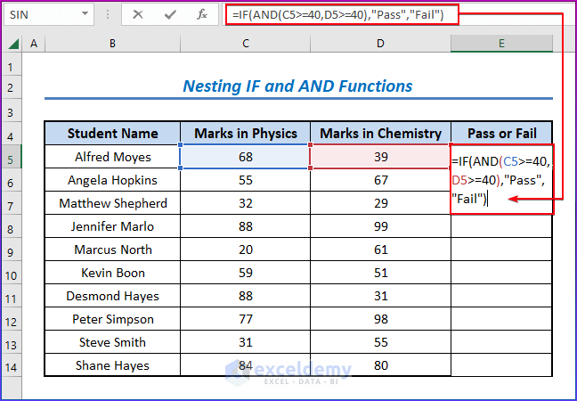
- Drag the Fill Handle to copy this formula to the rest of the cells.
- You can see the students who have passed both subjects have been judged as Pass.
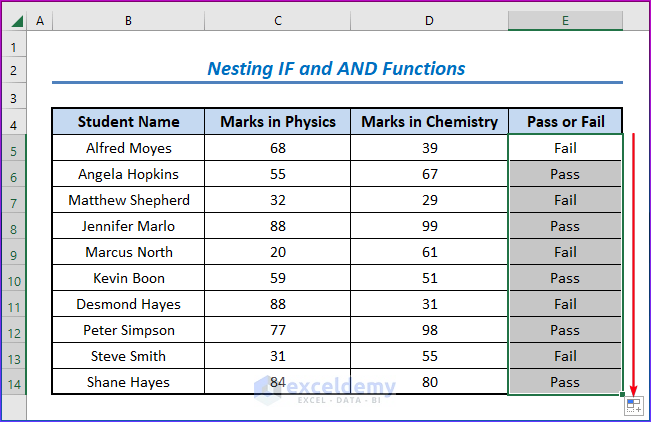
- C4>=40 returns TRUE if the mark in cell C4 (Mark in Physics) is greater than or equal to 40, or returns FALSE otherwise. Same goes for D4>=40.
- AND(C4>=40,D4>=40) returns TRUE only if both cells C4 and D4 contains values of 40 or greater.
- Finally, IF(AND(C4>=40,D4>=40),”Pass”,”Fail”) returns “Pass” if it encounters a TRUE or “Fail” if it doesn’t.
Method 3 – Using Nested IF Function for AND Type Criteria Between Multiple Ranges
Let’s repeat the same example as in Method 2 without AND.
Steps:
- Select the E5 cell and enter this formula:
=IF(C5>=40,IF(D5>=40,"Pass","Fail"),"Fail")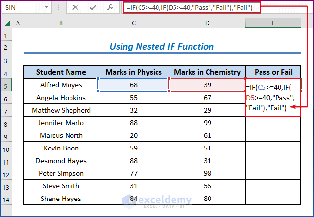
- Drag the Fill Handle to copy this formula to the rest of the cells.
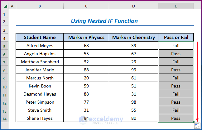
- If C4>=40 is TRUE, the formula enters into IF(D4>=40,”Pass”,”Fail”). If not, it returns “Fail”.
- Then if D4>=40 is also TRUE, it returns “Pass”; otherwise, it returns “Fail”.
- Thus, the formula returns “Pass” only if a student passes in both subjects.
Using Excel IFS Function Instead of IF for AND Type Criteria Between Multiple Ranges
Let’s use the same failing criteria as in Method 1.
Steps:
- Select the E5 cell and enter this formula:
=IFS(C5<40,"Fail",D5<40,"Fail",TRUE,"Pass")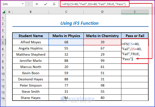
- Drag the Fill Handle to copy this formula to the rest of the cells.
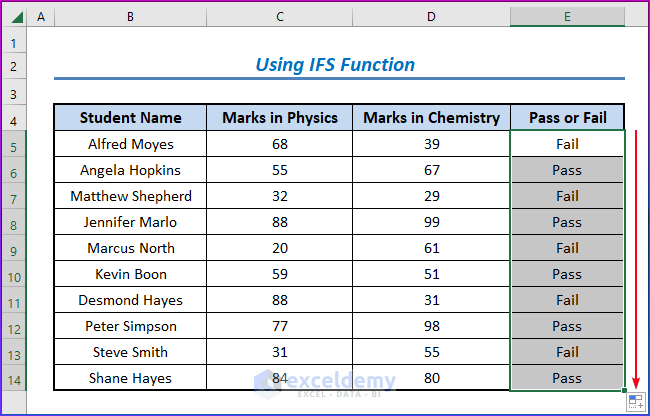
- The IFS function returns the value corresponding with the first TRUE argument. It returns a N/A error if it doesn’t find a result.
- If C4<40, it returns “Fail”. If not, then it checks whether D4<40. If the second check is TRUE, it returns “Fail”.
- If D4<40 is also FALSE, then it encounters a TRUE and returns “Pass”.
Read More: How to Use IF Function with Multiple Conditions in Excel
Download Practice Workbook
You may download the following Excel workbook to practice these methods.
Related Articles
<< Go Back to Excel IF Function | Excel Functions | Learn Excel
Get FREE Advanced Excel Exercises with Solutions!

