Excel ISTEXT Function: Syntax and Argument
In this section, we will explain the syntax and argument of the ISTEXT function.
ISTEXT Function of Excel (Quick View)
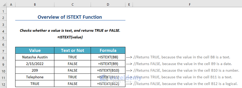
Summary:
Checks whether a value is text or not, if text, returns a TRUE. Otherwise, FALSE.
Works for both Array and Non-Array values.
Available from Excel 2003.
Syntax:
The Syntax of the ISTEXT function is:
=ISTEXT(value)
Argument:
| Argument | Required or Optional | Value |
|---|---|---|
| value | Required | The value we want to know is whether it is text or not. It can be any value or an array of values. |
Return Value:
Returns a Boolean value (TRUE or FALSE). TRUE if the value is a text, FALSE otherwise.
Method 1 – Use the ISTEXT Function
Steps:
- Select a new cell, C5, where you want to keep the result.
- Use the formula given below in the C5 cell.
=ISTEXT(B5)- Press ENTER.
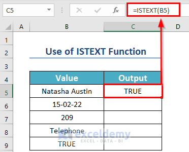
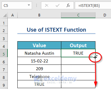
- Drag the Fill Handle icon to AutoFill the corresponding data in the rest of the cells C6:C9. Or you can double-click on the Fill Handle icon.
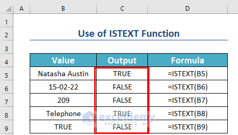
As a result, you will get the following output.
Method 2 – Check whether an Answer Is Valid or Not
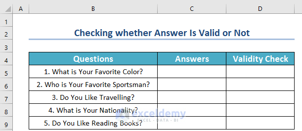
Now, look at the dataset below. Here, we have five questions in a column and empty spaces left for the answers.
Furthermore, we have kept an additional column called Validity Check. Each time you enter the answer to a question, it will show whether the answer is valid or invalid.
So, how to do that?
Steps:
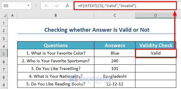
- Enter the following formula in cell D5:
=IF(ISTEXT(C5),"Valid","Invalid")- Then, press ENTER.
As you enter a text answer, it is showing as valid.
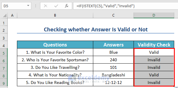
- Drag the Fill Handle icon to AutoFill the corresponding data in the rest of the cells C6:C9.
If you enter anything other than text as the answer, it will show invalid.
Formula Explanation:
- Firstly, ISTEXT(C5) returns a TRUE if the value in cell C5 is a text, otherwise FALSE.
- Secondly, IF(ISTEXT(C5),”Valid”,”Invalid”) returns “Valid” if it sees a TRUE, and for a FALSE it returns “Invalid”.
The same goes for the rest of the cells.
If any answer is entered as anything other than a text, it returns “Invalid”. And when the answer is a text value, it returns “Valid”.
Method 3 – Employing the ISTEXT Function to Count Cells Containing Text
Look at the dataset below. It contains the joining dates and designations of some employees of Dynamo Group.
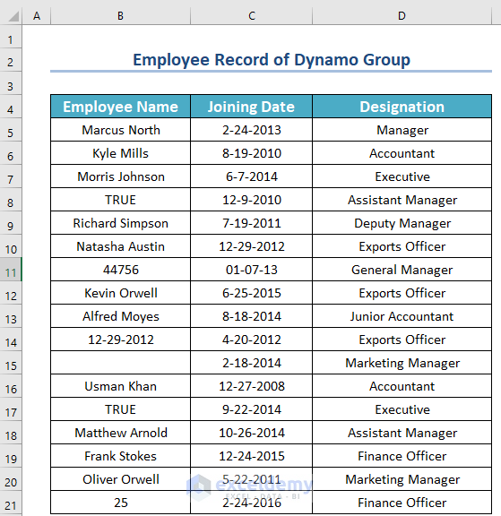
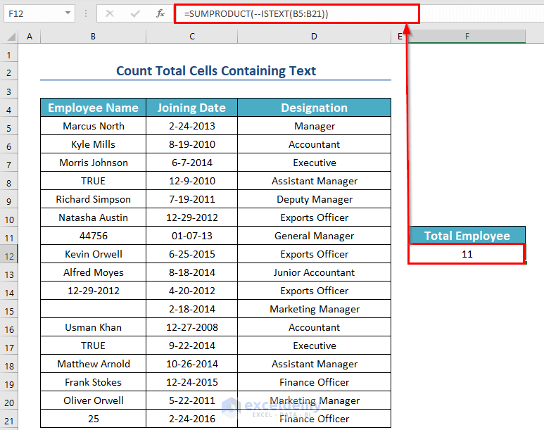
Now, say you want to know how many employees entered their valid names. Or, suppose we find out the total number of enrolled employees. Here, we will use SUMPRODUCT and ISTEXT functions.
- Enter the following formula in cell F12:
=SUMPRODUCT(--ISTEXT(B5:B21))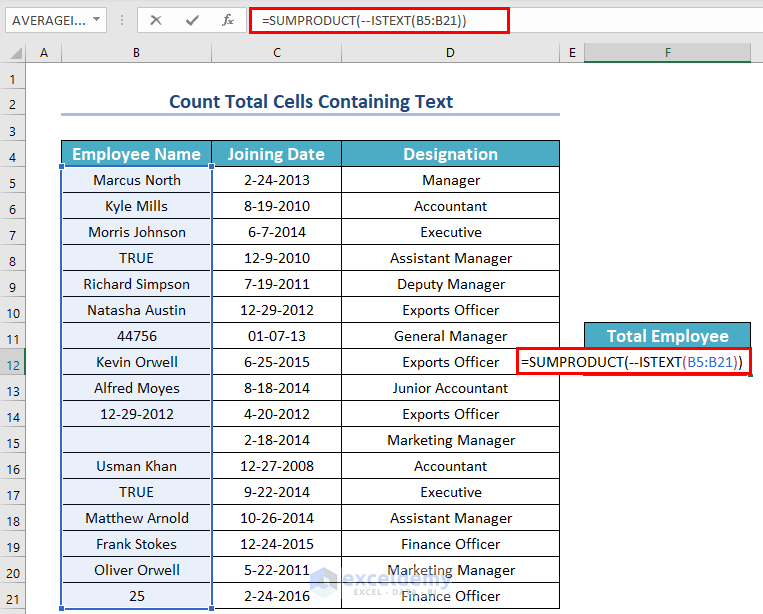
Formula Explanation:
- Firstly, ISTEXT(B5:B21) will check whether the values of B5:B21 cells are text or not. If the cell contains text then it will return TRUE otherwise FALSE.
- Secondly, the Double Hyphen (–) converts the logical values into binary numbers.
- Thirdly, the SUMPRODUCT function will count all those numbers.
- Press ENTER to get the result.
Method 4 – Using the ISTEXT Function in Data Validation
Steps:
- Select cells B5:B11 where you want to insert only one kind of cell value (text values).
- From the Data tab >> go to the Data Tools option.
- From the Data Validation feature >> choose Data Validation… option.
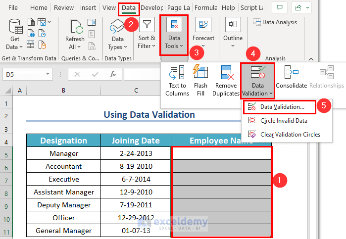
A dialog box named Data Validation will appear.
- From the Settings menu >> choose Custom in the Allow: box.
- Enter the following formula in the Formula box:
=ISTEXT(D5:D11)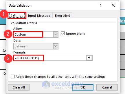
- From the Error Alert menu.
- Enter the following text in the Error message box.
Please Enter Name- Press OK to make the changes.
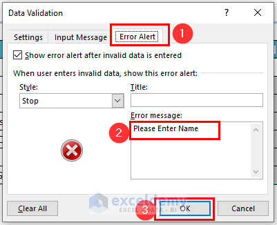
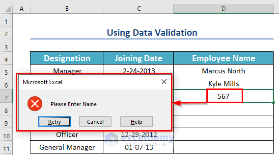
As a result, if you enter any number or date in the D5:D11 cells, you will get the following notice from Microsoft Excel:
Method 5 – Employing Conditional Formatting with ISTEXT Function
Steps:
- Select cell B5, where you want to apply the Conditional Formatting to color the cell containing text value.
- From the Home tab >> go to the Conditional Formatting command.
- Choose the Highlight Cells Rules feature >> select More Rules…
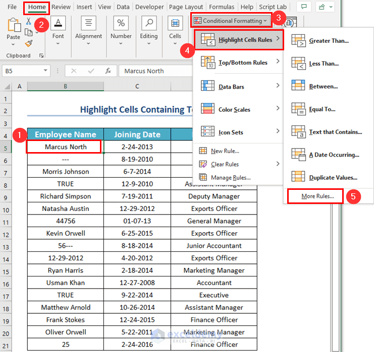
A dialog box named New Formatting Rule will appear.
- From that dialog box,>> select Use a formula to determine which cells to format.
- Enter the following formula in the Format values where this formula is true: box.
=ISTEXT(B5)Here, the ISTEXT function will check whether the value of cell B5 is text or not. If the cell contains text, then it will return TRUE otherwise FALSE. One thing: Don’t use absolute references in the formula. Then, you won’t be able to use the same format in other cells.
- Go to the Format menu.

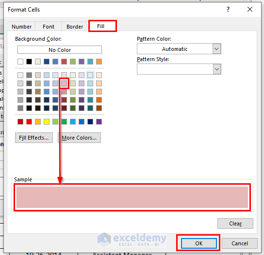
A dialog box named Format Cells will appear.
- From the Fill option >> choose any of the colors. Here, we have chosen Light Red. Also, you can see the sample instantly. In this case, try to choose any light color. Because the dark color may hide the inputted data, you may need to change the Font Color.
- Press OK to apply the formation.
- Press OK on the New Formatting Rule dialog box. Here, you can see the sample instantly in the Preview box.
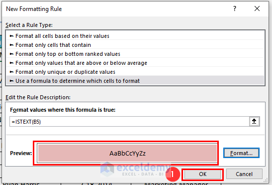
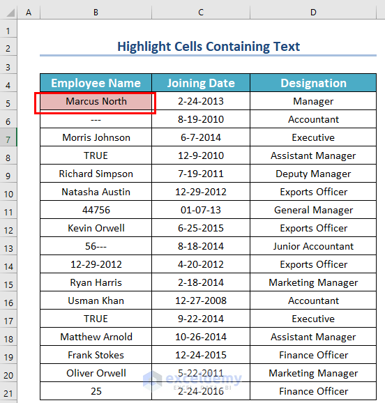
As a result, you will see that cell B5 is colored.
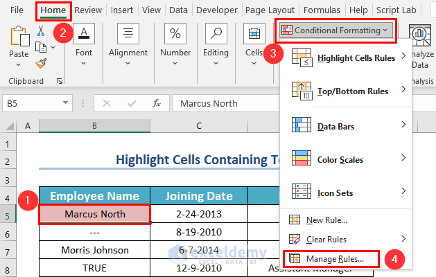
- Select the B5 cell where you have applied the Conditional Formatting.
- From the Home tab >> go to the Conditional Formatting command.
- Choose Manage Rules…
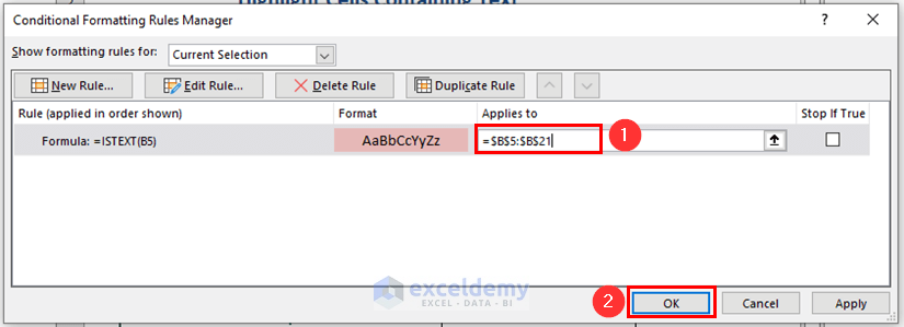
You will see another dialog box named Conditional Formatting Rules Manager.
- Select B5:B21 cells in the Applies to box.
- Press OK.
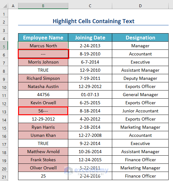
You will see all the cells that contain text as cell values are highlighted. But, if you notice, you will see that Excel counts the Hyphen as text. Furthermore, with numbers, if you insert any alphabet or symbol, Excel will also count them as text.
Method 6 – Check Whether the Date Is Correctly Entered or Not
Steps:
- Enter the following formula in the first cell of a new column and then press ENTER.
=IF(ISTEXT(C5),"Not Correctly Entered","Correctly Entered")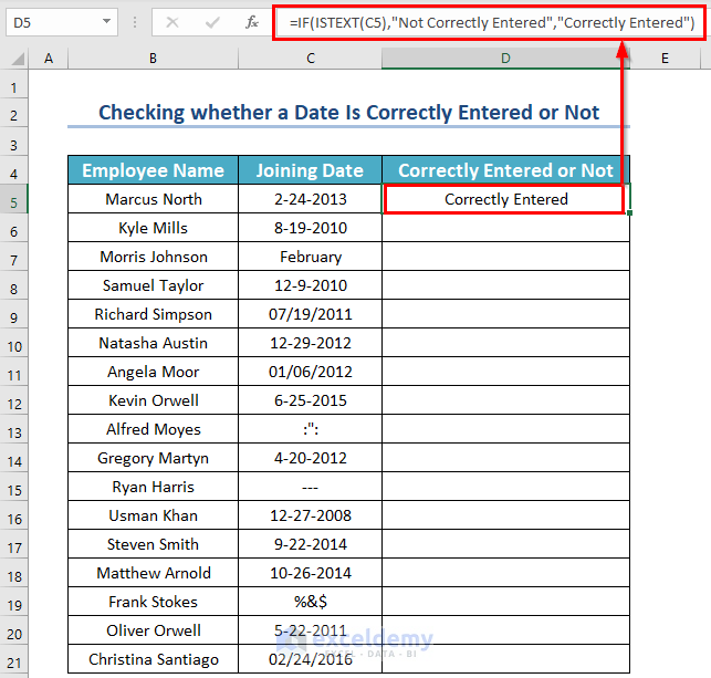
- Drag the Fill Handle icon.
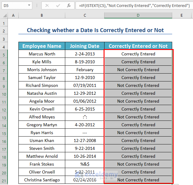
A few of the dates are not correctly entered. They are text values.
Formula Explanation:
- Firstly, ISTEXT(C5) returns a TRUE if the value in cell C5 is a text, otherwise FALSE.
- Secondly, IF(ISTEXT(C5),”Not Correctly Entered”,”Correctly Entered”) returns “Not Correctly Entered” if it sees a TRUE, and for a FALSE it returns “Correctly Entered”.
- Do the same for the rest of the cells.
If any date is entered as a text, a “Not Correctly Entered” is returned.
Method 7 – Use IF, SUMPRODUCT & ISTEXT Functions
Steps:
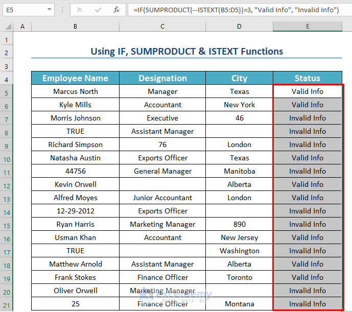
- Select a different cell, E5, where you want to see the Status.
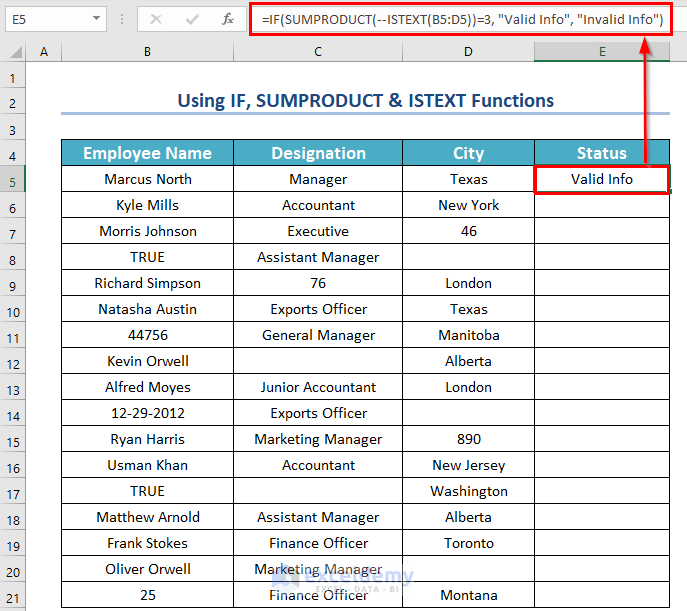
- Use the corresponding formula in cell E5:
=IF(SUMPRODUCT(--ISTEXT(B5:D5))=3, "Valid Info", "Invalid Info")- Press ENTER.
Formula Explanation:
- Firstly, ISTEXT(B5:D5) will check whether the values of B5:D5 cells are text or not. If the cell contains text then it will return TRUE otherwise FALSE.
- Output: {TRUE,TRUE,TRUE}.
- Secondly, the Double Hyphen (–) converts the logical values into binary numbers.
- Output: {1,1,1}.
- Thirdly, the SUMPRODUCT function will count all those numbers.
- Output: 3.
- Fourthly, the IF function will check whether the above output is equal to 3 or not. If the logical test is true then it will return “Valid Info” otherwise “Invalid Info”.
- Output: “Valid Info”.
- Drag the Fill Handle icon to AutoFill the corresponding data in the rest of the cells E6:E21.
As a result, you will see all the statuses.
Method 8 – Use ISTEXT as an Array Formula in Excel
Steps:
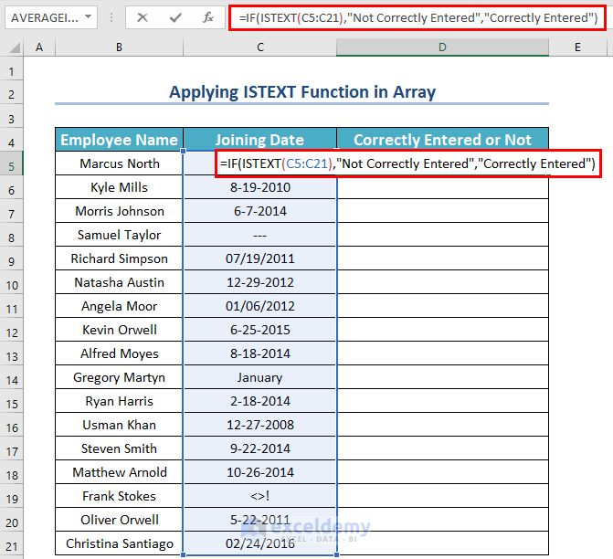
- Enter the following formula in cell D5:
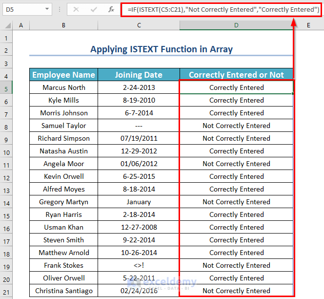
=IF(ISTEXT(C5:C21),"Not Correctly Entered","Correctly Entered")(Do not forget to press CTRL + SHIFT + ENTER unless you are in Office 365.)
Formula Explanation:
- Actually, IF(ISTEXT(C5:C21),”Not Correctly Entered”,”Correctly Entered”) is a combination of 17 single formulas.
- So, at first, it breaks the formula into 17 single formulas.
- Then, it checks whether each value in the array C5 to C21 is a text or not.
- For those texts, it returns “Not Correctly Entered”.
- And for those not texts, it returns “Correctly Entered”.
- Press ENTER, and you will get the result.
How to Use Combined Functions to Identify Cells Containing Certain Text in Excel
Steps:
- Enter this formula in the first cell of a new column and then press ENTER.
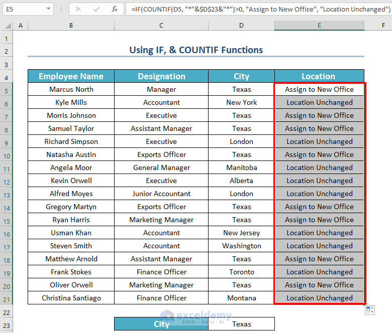
=IF(COUNTIF(D5, "*"&$D$23&"*")>0, "Assign to New Office", "Location Unchanged")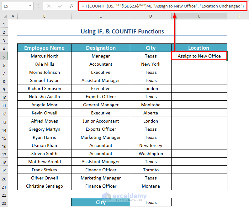
Formula Explanation:
- COUNTIF(D5, “*”&$D$23&”*”)—> here, D5 is the cell range and “*”&$D$23&”*” is the criteria.So, the COUNTIF function will check whether the text value is Texas. And if the cell hold Texas as value then it will count the cell.
- Output: 1.
- IF1>0, “Assign to New Office”, “Location Unchanged”)—> Here, the IF function will check whether the previous value is greater than 0 or not. If the value is greater than 0 then the IF function will return “Assign to New Office”. Otherwise, it will return “Location Unchanged”.
- Output: Assign to New Office.
- Drag the Fill Handle icon to AutoFill the corresponding data in the rest of the cells E6:E21.
As a result, you will see all the statuses.
Common Errors with Excel ISTEXT Function
Here, we will explain the common errors of the ISTEXT function and the reasons for occurring such errors.
- The ISTEXT function itself doesn’t give an error. It always returns either TRUE or FALSE. The ISTEXT function just checks whether the cell value is text or something else.
- However, for this ISTEXT function, you may face other problems with other functions. Like, you are using a formula, and in that formula, you are using a cell that contains text. So, the ISTEXT function will simply return TRUE, and in Boolean, it will convert to 1, but you will get an error with that formula as your reference cell was text, not number.
Practice Section
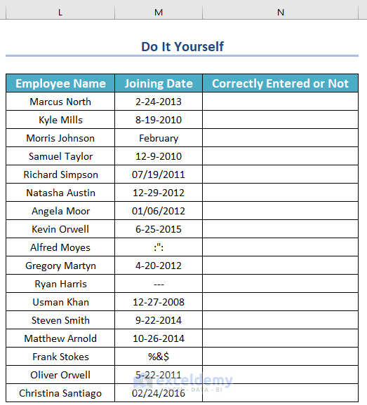
Now, you can practice the methods.
Download the Practice Workbook
Download the Workbook to practice.
<< Go Back to Excel Functions | Learn Excel
Get FREE Advanced Excel Exercises with Solutions!

