Suppose a bookshop sells books both online and in stores. However, they have two booklists, one featuring books available for online sale and the other books available for sale in the store. Each list is stored on a separate sheet in an Excel workbook.
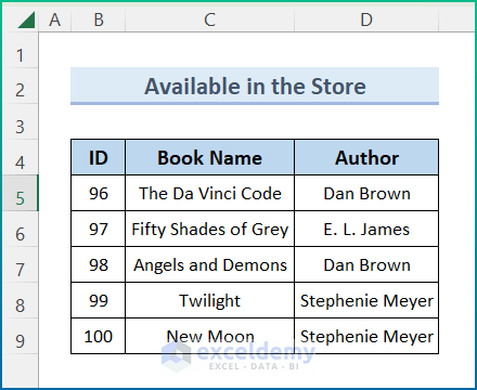
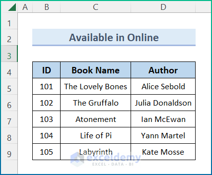
In this tutorial, we will use the VLOOKUP function in 3 distinct ways to combine these two lists of books on different sheets into one new list.
Method 1 – Lookup Across Multiple Sheets in Excel with IFERROR Function
We can use the IFERROR function together with the VLOOKUP function to combine the “Store” and “Online” worksheet data.
Steps:
- In cell C5 enter the following formula:
=IFERROR(VLOOKUP(B5,Store!$B$5:$D$9,2, FALSE), IFERROR(VLOOKUP(B5,Online!$B$5:$D$9, 2, FALSE), "Not found"))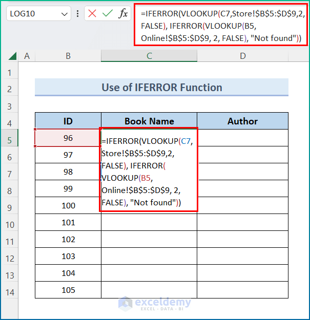
- Press ENTER.
- Drag the Fill Handle icon to the end of the Book Name column.
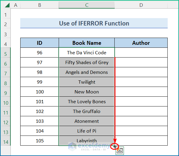
␥ Formula Breakdown
Syntax: IFERROR(VLOOKUP(…), IFERROR(VLOOKUP(…), …, "Not found"))
- B5 ▶ picks up an ID, which will work as a search key.
- Store!$B$5:$D$9 ▶ searches within the range from B5 to D9 in the Store worksheet.
- Online!$B$5:$D$9 ▶ searches within the range from B5 to D9 in the Online worksheet.
- 2 ▶ indicates the Book Name column to retrieve the book names from.
- FALSE ▶ specifies exact matches are required while searching.
=IFERROR(VLOOKUP(B5,Store!$B$5:$D$9,2, FALSE), IFERROR(VLOOKUP(B5,Online!$B$5:$D$9, 2, FALSE), "Not found"))▶ returns the book name with ID no. 96.
- Similarly, to complete the Author column, enter the following formula in cell D5:
=IFERROR(VLOOKUP(B5,Store!$B$5:$D$9,3, FALSE), IFERROR(VLOOKUP(B5,Online!$B$5:$D$9, 3, FALSE), "Not found"))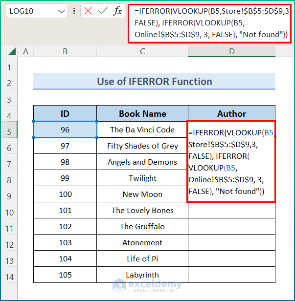
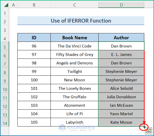
- Press Enter and utilize the AutoFill tool to fill the entire column.
Method 2 – Combining INDIRECT, INDEX and COUNTIF Functions
We can lookup across multiple sheets using the INDIRECT function instead of the IFERROR function. However, although the INDIRECT function provides a lot more flexibility while retrieving data across multiple sheets, its syntax is more complicated. We’ll also make use of the COUNTIF, INDEX, and MATCH functions here.
Steps:
- In cell C5, enter the following formula:
=VLOOKUP($B5,INDIRECT("'"&INDEX($F$5:$F$6,MATCH(TRUE,COUNTIF(INDIRECT("'"&$F$5:$F$6&"'!$B5:$B9"),$B5)>0,0))&"'!$B$5:$D$9"),2,0)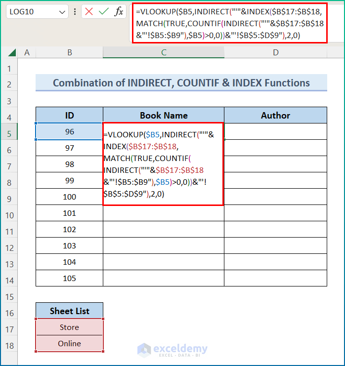
- Press ENTER.
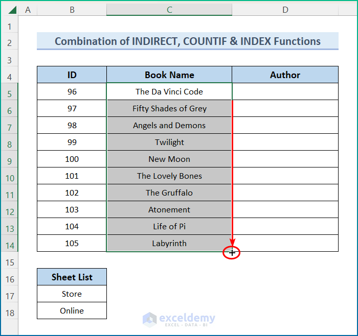
- Drag the Fill Handle icon to the end of the Book Name column.
␥ Formula Breakdown
Syntax: VLOOKUP(lookup_value, INDIRECT("'"&INDEX(Lookup_sheets, MATCH(TRUE, --(COUNTIF(INDIRECT("'" & Lookup_sheets & "'!lookup_range"), lookup_value)>0), 0)) & "'!table_array"), col_index_num, FALSE)
- Lookup_value ▶ $B5 ▶ the search keyword based on which we conduct the search.
- Lookup_sheets ▶ $F$5:$F$6 ▶ the cell address of the list of sheets throughout which we will perform the lookup.
- Lookup_range ▶ $B5:$B9 ▶ the range within which our lookup value resides.
- Table_array ▶ $B$5:$D$9 ▶ the range of the whole data table.
- Column_index_number ▶ 2 ▶ the column number from where we pull our desired data.
- Similarly, to make the Author column complete, use the formula below in cell D5:
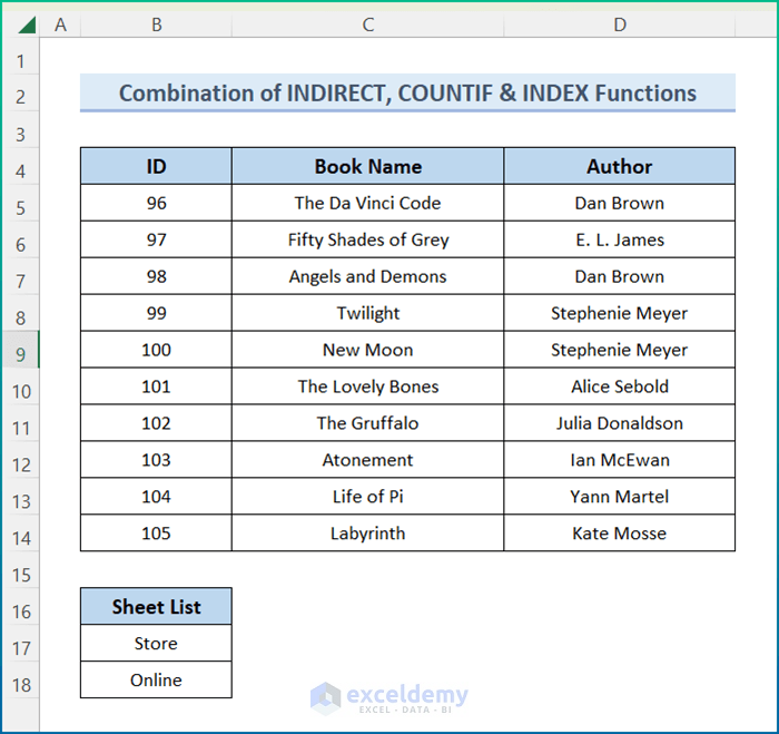
=VLOOKUP($B5,INDIRECT("'"&INDEX($F$5:$F$6,MATCH(TRUE,COUNTIF(INDIRECT("'"&$F$5:$F$6&"'!$B5:$B9"),$B5)>0,0))&"'!$B$5:$D$9"),3,0)- Utilize the AutoFill tool and the final output will appear as in the image below.
Method 3 – Combining IF and ISNA Functions
This method is suitable if you only have a few datasheets to pull data from. If you have to deal with many sheets, we recommend you use one of the above Methods, because this one gets much more complicated as the number of sheets increases.
Steps:
- In cell C5, enter the formula below:
=IF(ISNA(VLOOKUP($B5,Store!$B$5:$D$9,2,0)),VLOOKUP($B5,Online!$B$5:$D$9,2,0),IF(ISNA(VLOOKUP($B5,Online!$B$5:$D$9,2,0)),VLOOKUP($B5,Store!$B$5:$D$9,2,0)))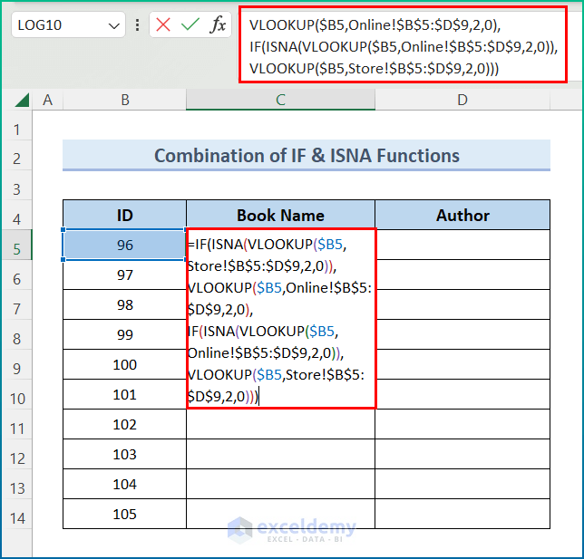
- Press ENTER.
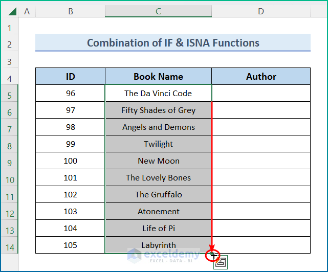
- Drag the Fill Handle icon to the end of the Book Name column.
␥ Formula Breakdown
Syntax: IF(ISNA(VLOOKUP(lookup_value,table_array,col_index_number,0)),value_if_true,value_if_false)
- Lookup_value ▶ $B5 ▶ the search keyword based on which we conduct the search.
- Table_array ▶ $B$5:$D$9 ▶ the range of the whole data table.
- Column_index_number ▶ 2 ▶ the column number from where we pull our desired data.
- ISNA(VLOOKUP($B5,Store!$B$5:$D$9,3,0)) ▶ searches for the cross-matching of the ID (referred by $B5) within the range $B$5:$D$9.
- IF(ISNA(VLOOKUP($B5,Store!$B$5:$D$9,3,0)),VLOOKUP($B5,Online!$B$5:$D$9,3,0) ▶ If ISNA(VLOOKUP($B5,Store!$B$5:$D$9,3,0)) is true then the corresponding book name is pulled using VLOOKUP($B5,Online!$B$5:$D$9,3,0).
- If the part IF(ISNA(VLOOKUP($B5,Store!$B$5:$D$9,3,0)),VLOOKUP($B5,Online!$B$5:$D$9,3,0) becomes false then we enter into IF(ISNA(VLOOKUP($B5,Online!$B$5:$D$9,3,0)),VLOOKUP($B5,Store!$B$5:$D$9,3,0)).
- IF(ISNA(VLOOKUP($B5,Online!$B$5:$D$9,3,0)),VLOOKUP($B5,Store!$B$5:$D$9,3,0)) ▶ If ISNA(VLOOKUP($B5,Online!$B$5:$D$9,3,0)) becomes true then we pull the book name using VLOOKUP($B5,Store!$B$5:$D$9,3,0)).
- Similarly, to make the Author column complete, use the following formula:
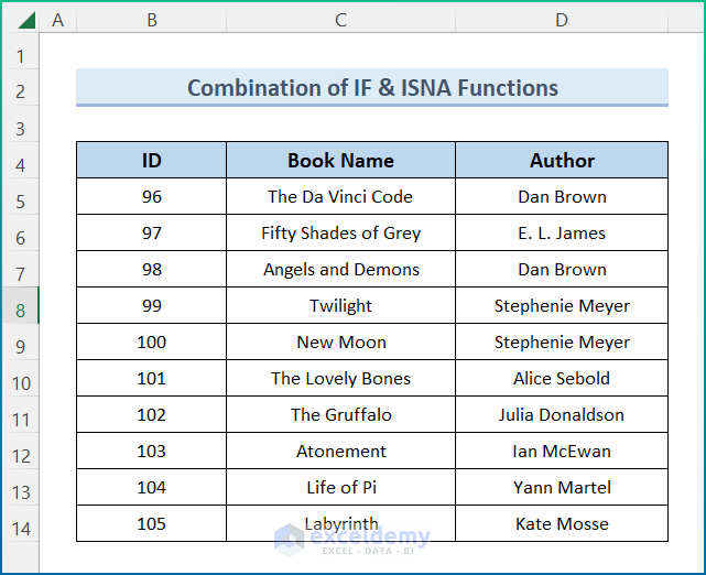
=IF(ISNA(VLOOKUP($B5,Store!$B$5:$D$9,3,0)),VLOOKUP($B5,Online!$B$5:$D$9,3,0),IF(ISNA(VLOOKUP($B5,Online!$B$5:$D$9,3,0)),VLOOKUP($B5,Store!$B$5:$D$9,3,0)))The desired output is returned.
Things to Remember
- The lookup value should always be in the first column within the table array.
- Use Ctrl + Shift + Enter together to complete array formulas if you are not using Excel 365.
- Be precise with the syntax of the functions to avoid errors.
- Insert data ranges carefully into the formulas to avoid errors and incorrect results.
Download the Practice Workbook
<< Go Back to Lookup | Formula List | Learn Excel
Get FREE Advanced Excel Exercises with Solutions!

