How to Lookup Next Largest Value in Excel (4 Easy Ways)

In this article, we will demonstrate various methods to find the next largest value in a sorted or unsorted dataset.

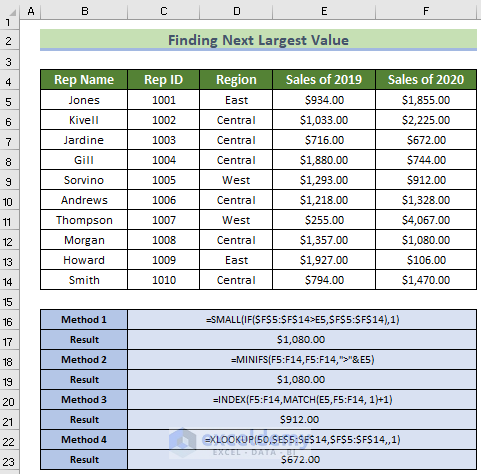
Overview of Excel Lookup Next Largest Value

To demonstrate our methods, we’ll use the following dataset. The values are in unsorted form.

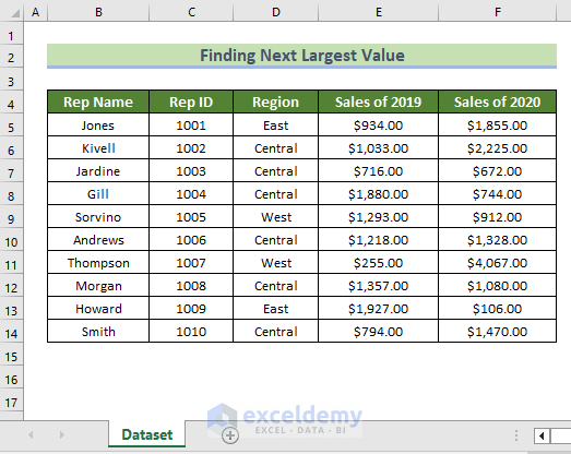
Dataset for Excel Lookup Next Largest Value

We will find the next largest sales value from Sales of 2020 according to the value selected in Sales of 2019.

We used the Microsoft Office 365 version in this tutorial.

Method 1 – Using the SMALL Function

If the dataset is unsorted, we can use the SMALL and IF functions to find the next largest value.

Steps:

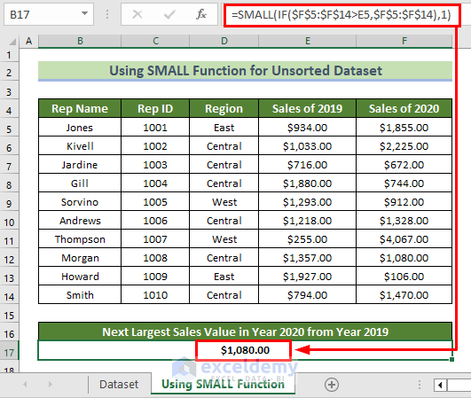
Select cell B17 and enter the following formula:

=SMALL(IF($F$5:$F$14>E5,$F$5:$F$14),1)

Press ENTER.

Formula Breakdown

IF($F$5:$F$14>E5,$F$5:$F$14) → checks if there are numbers greater than the lookup value.
- $F$5:$F$14>E5 → is the logical test where the IF function will check for the next largest value.
  - $F$5:$F$14 → is the lookup array where the value will be searched.
  - E5 → contains the value to be searched.
- $F$5:$F$14 → is the condition using which the values greater than the lookup value will be stored. If the condition is not met, FALSE will be stored.
  - Output → array of numbers that satisfies the condition and FALSE text.
- SMALL(IF($F$5:$F$14>E5,$F$5:$F$14),1) → becomes
  - SMALL(array,1) → returns the next largest value using the position of the value on the array that the IF function has created.
    - array is where the values satisfying the IF function are stored.
    - 1 is the position of the value to return.
      - Output → $1080.00

Method 2 – Using the MINIFS Function

The MINIFS function is an Excel function that is a combination of MIN and IFS functions.

Steps:

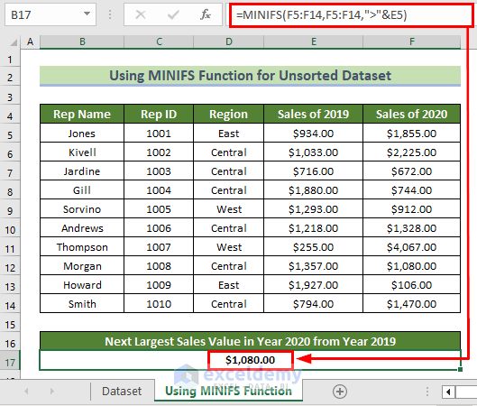
Select cell B17 and enter the following formula:

=MINIFS(F5:F14,F5:F14,">"&E5)

Press ENTER.

Formula Breakdown

MINIFS(F5:F14, F5:F14,”>”&E5) → finds the next largest value according to the minimum range, criteria range, and criteria.
- F5:F14 → is the minimum range where the MINIFS function will search for value.
- F5:F14 → is the criteria range.
- “>”&E5 → is the criteria for finding the values larger than the provided value.
  - Output → $1080.00

Match 3 – Using the INDEX and MATCH Functions with the Sort Feature

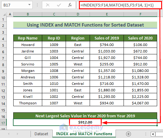
If the dataset is sorted in ascending order, we can use the INDEX and MATCH functions to find the next largest value.

Steps:

Select cell B17 and enter the following formula:

=INDEX(F5:F14,MATCH(E5,F5:F14, 1)+1)

Press ENTER.

Formula Breakdown

MATCH(E5, F5:F14, 1)+1 → searches for the cell location using these arguments:
- E5 is the searched value.
- F5:F14 is the array in which the value is searched.
- 1 means the MATCH function will search for values less than the lookup value.
- +1 will go to the next position the MATCH function has found.
  - Output → 4
- INDEX(F5:F14, MATCH(E5, F5:F14, 1)+1) → becomes
  - INDEX(F5:F14,4) → searches for the cell value in the cell position found by the MATCH function.
    - F5:F14 → is the array where the INDEX function will search for the value.
    - 4 is the row number where the value is.
      - Output → $912.00

Method 4 – Using XLOOKUP Function to Find Corresponding Value

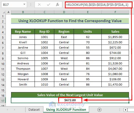
The XLOOKUP function works a little differently from the functions used above. It will search for the next largest value when there is no exact match found and return its corresponding value. In this example, if we enter a non-exact Units value, the XLOOKUP function will return the next largest Sales value.

Steps:

Select cell B17 and enter the following formula:

=XLOOKUP(50,$E$5:$E$14,$F$5:$F$14,,1)

Press ENTER.

Formula Breakdown

XLOOKUP(50,$E$5:$E$14,$F$5:$F$14,,1) → searches for an exact match or greater value and returns a corresponding value.
- 50 is the searched value.
- $E$5:$E$14 is the array where the XLOOKUP function will search for the value.
- $F$5:$F$14 is the return array from where the corresponding value will be returned.
- 1 means the function will search for an exact match or larger value.
  - Output → $672.00