Mapping Data from Another Sheet in Excel (6 Useful Methods)

Suppose you have the following two datasets.

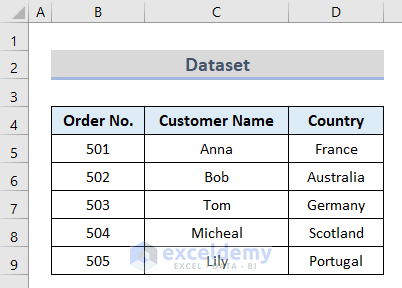
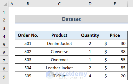
Method 1 – Link Cells for Mapping Data from Another Sheet in Excel

Steps:

• Insert an Equal (=) sign in an appropriate cell (F5 in this example).

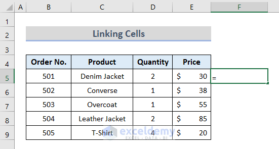
• On the source dataset worksheet, click the appropriate cell (D5).

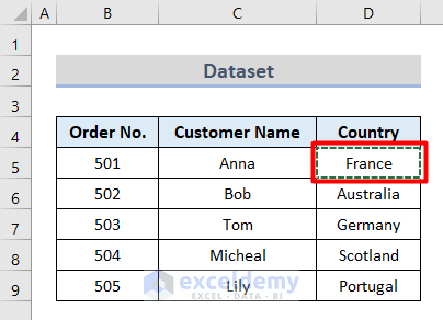
• Return to the previous worksheet. It should now show information about the cell it’s linked to.
• Press Enter.

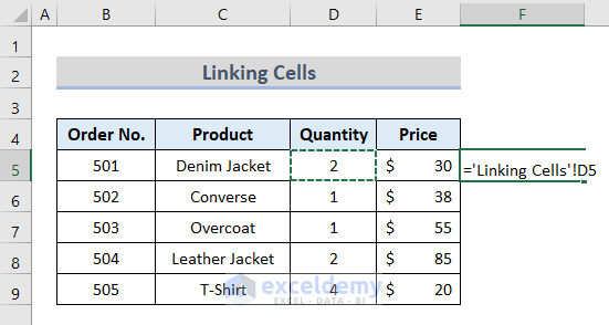
The cell should show the information from the source cell.

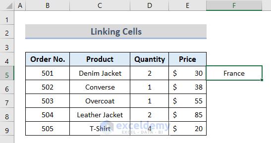
• Use the AutoFill tool to copy the link to the rest of the column.

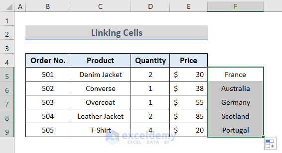
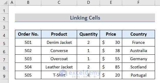
• Follow the same process to link the header title.
• Format the linked column to match the rest of the sheet if necessary.

Read More: How to Create Mind Map from Data in Excel

Method 2 – Use the VLOOKUP Function to Map Data in Excel

Steps:

• Insert the following formula in the appropriate cell (F5 in our example).

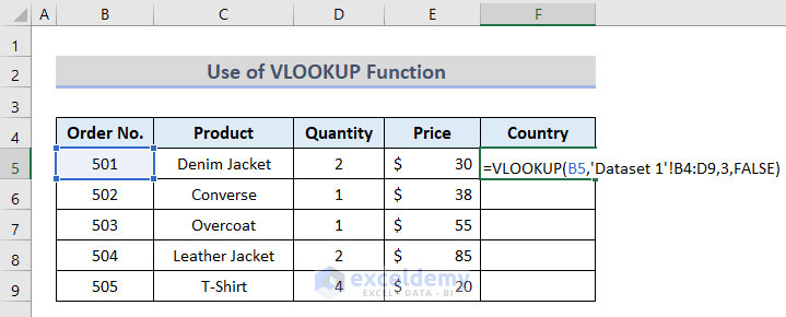
The Lookup Value is the cell that both worksheets have in common (B5).

The Table Array is the source data (‘Dataset 1’!B4:D9).

The Column_Index_Num is how many columns Excel has to count over to find the required information (3).

Exact match is False in this example.

• Press Enter.

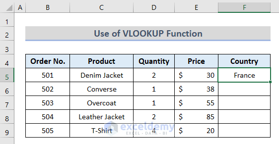
• Use the AutoFill tool to copy the formula to the rest of the column.

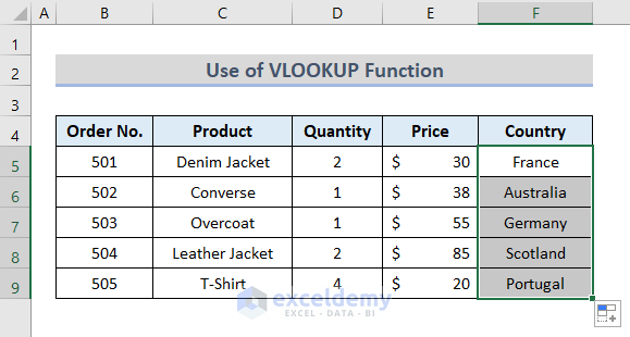
Method 3 – Pull Data from Another Sheet with INDEX-MATCH Function

Steps:

• Insert the following formula in the appropriate cell (G14).

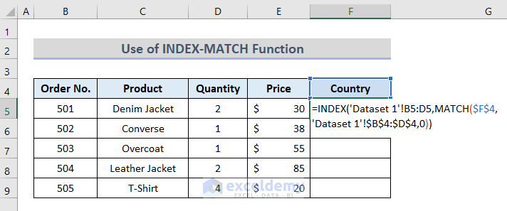
The INDEX function returns the value, and the MATCH function helps to find the exact match from the source.

• Press Enter.

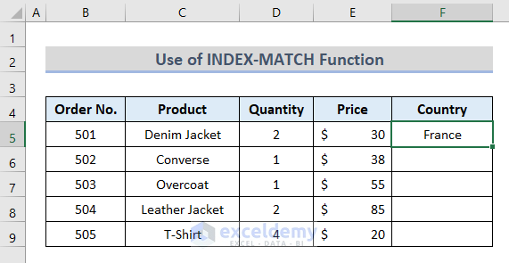
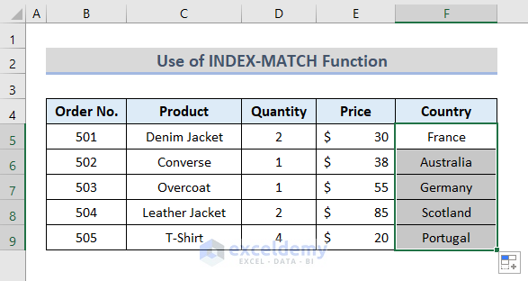
• Use the AutoFill tool to copy the formula to the rest of the column.

Method 4 – Use the Advanced Filter to Map Data from a Different Sheet

Steps:

• Select the destination worksheet.
• Go to the Data tab and choose Advanced under the Sort & Filter group.

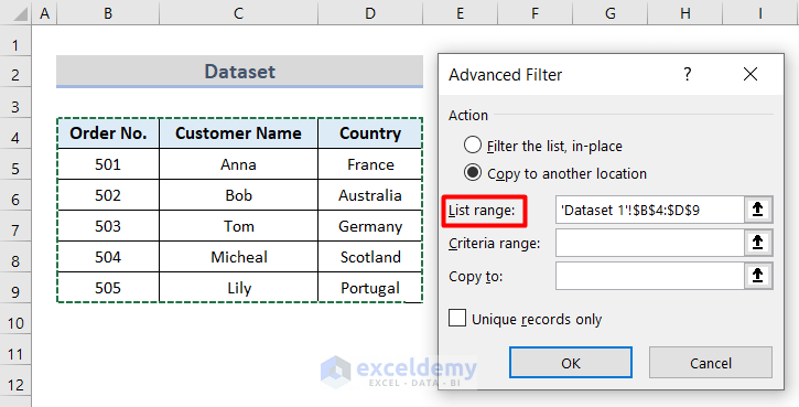
• An Advanced Filter window pops up.
• Choose the Copy to another location option.
• Input the appropriate range from the Dataset 1 worksheet into the List range box.

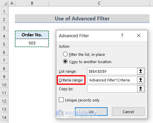
• Choose the Criteria range from the second sheet.

• Add the destination cell information in the Copy to box.

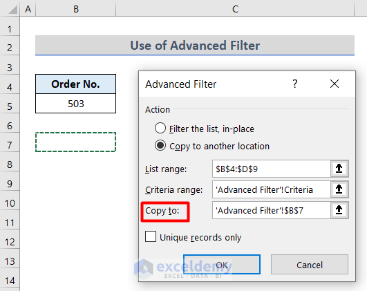
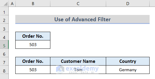
• Press OK.

Method 5 – Use Excel VLOOKUP & INDIRECT Functions for Mapping Data

Suppose you have the following two datasets:

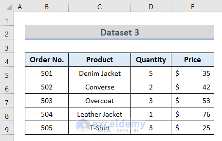
Steps:

• Open a new worksheet and put this formula in a blank cell (C5 in this example).

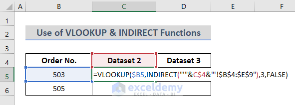
The INDIRECT function transforms the string into a name that Excel can understand and puts it in the table_array argument of VLOOKUP.

• Press Enter.

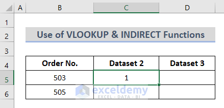
• Use the AutoFill tool to copy the formula to the rest of the column.

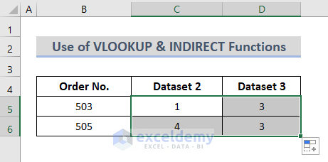
Method 6 – Map Data from Another Sheet with the HLOOKUP Function in Excel

Steps:

• Add the proper order to an empty cell beside the destination cells (F5:F9 in this example).

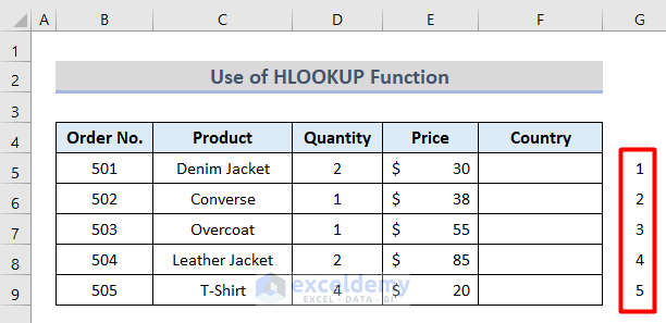
• Use this formula in the destination cell (F5).

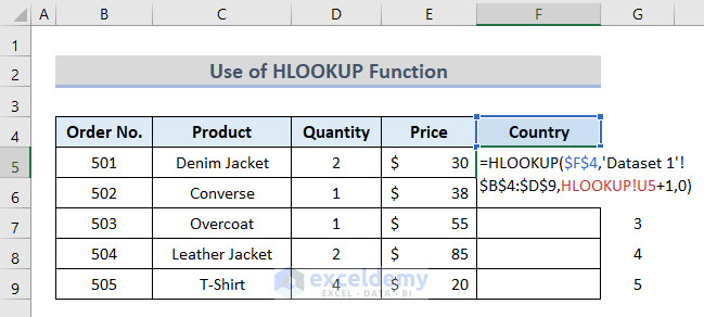
• Press Enter.

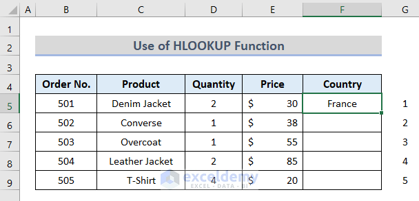
• Use the AutoFill tool to copy the formula to the rest of the column.

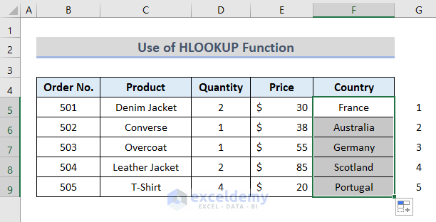
• Delete the order cells.

Download Workbook

Get the sample file here and practice it by yourself.

Related Articles

• How to Save Excel File As XML Data Mapping
• How to Map Data Using VLOOKUP in Excel

<< Go Back To Data Mapping in Excel | Importing Data in Excel | Learn Excel