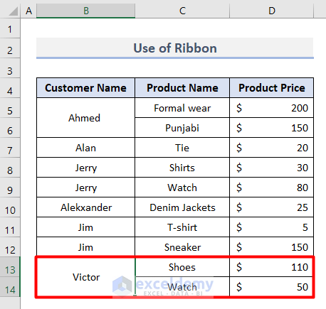
Our sample datasheet contains 3 columns: Customer Name, Product Name, and Product Price. Some Customer Names are repeated. We will merge those cells and show them in a single cell.
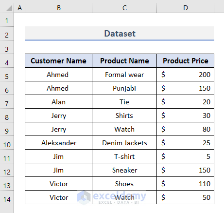
Method 1 – Merge Rows with the Same Value with Merge & Center
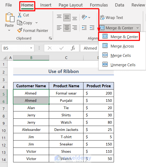
- Select the rows with the same value you want to merge.
- Open the Home tab and expand the Merge & Center option.
- Select Merge & Center.
- A dialogue box will pop up with a message that says Excel keeps the upper-left value.
- Click on OK.

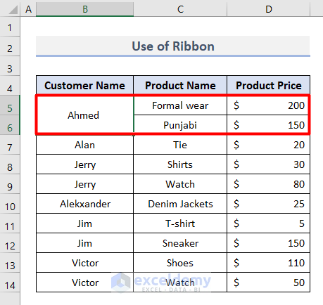
- You will get the merged rows where the value is in the center.
You can also merge rows specifying cells.
- Select the rows you want to merge.
- Open the Home tab and expand the Merge & Center option.
- Select Merge Cells from the drop-down menu.
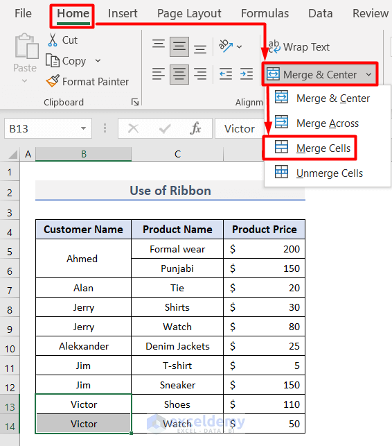
- It will merge the rows with the same value.
Method 2 – Apply the Consolidate Command to Merge Rows in Excel
- Select a cell where you want to keep merged rows with the same value. We separated the Customer Name and the Product Price columns and selected a cell from it.
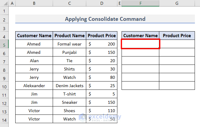
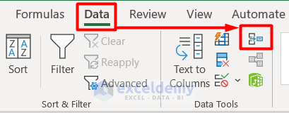
- Open the Data tab and select Consolidate under the Data Tools category.
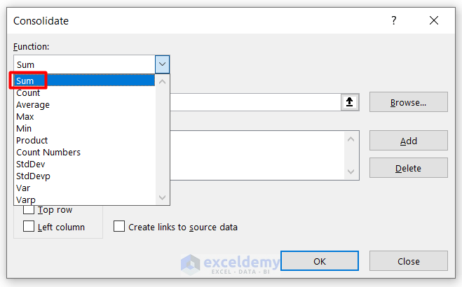
- A dialogue box will pop up from where you can select the functions given. We selected the SUM function.
- Take the Reference of the cell range B5:D14 as we want to consolidate them.
- Add this in All references.
- Check Left column as we’re merging the Customer Name values and summing by Product Price.
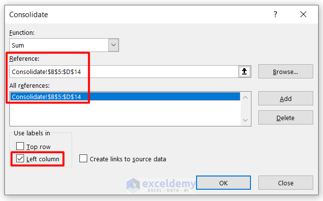
- Click on OK.
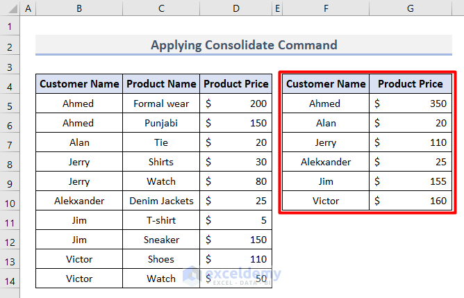
- You will get the merged values with the SUM of Product Price.
Method 3 – Use the IF Function to Merge Rows with the Same Value
- Select the cell range B5:B14 as we want to sort the Customer Names alphabetically.
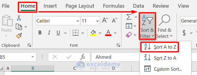
- Go to the Data tab and click on Sort & Filter.
- Choose Sort A to Z.
- Create a new column E titled Merged Rows with Same Values.
- Select cell E5 and insert this formula.
=IF(B5=B4,E4&", "&C5,C5)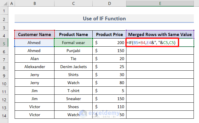
- The function will start comparing consecutive values. The first value doesn’t have anything above it so it returns just the value from that row.
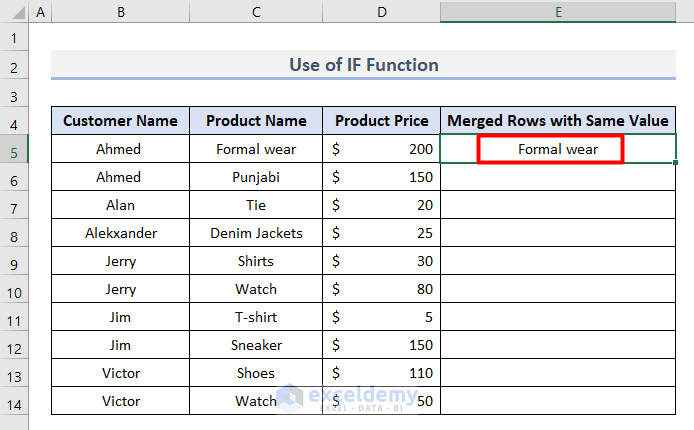
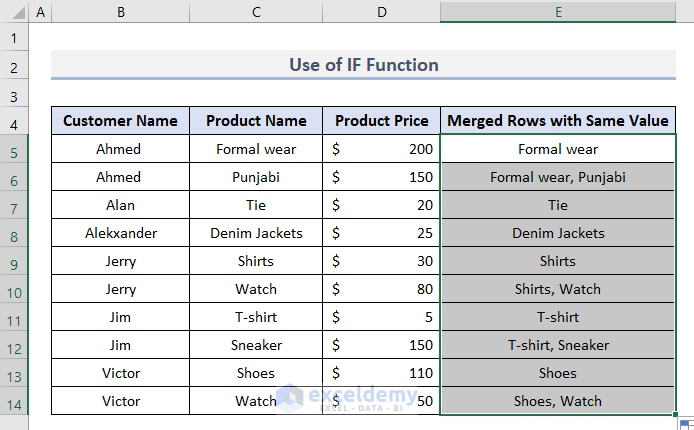
- Select the Cell E5 cell and double-click on the bottom-right corner to copy the formula for the rest of the cells.
- This shows the merged values of the same rows.
Method 4 – Merge Multiple Rows with the Same Value Using Excel VBA
- Sort the rows based on the cell you want to merge.
- We selected the Cell range B5:B14 as we want to sort by the Customer Name column.
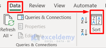
- Click on Sort from the Data tab.
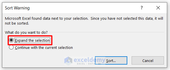
- The Sort Warning dialogue box will pop up.
- Choose the option Expand the selection and click on Sort.
- Select Customer Name as the Sort by option.
- Click on OK.
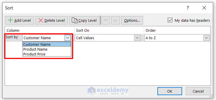
- This will provide the sorted values of the Customer Name.
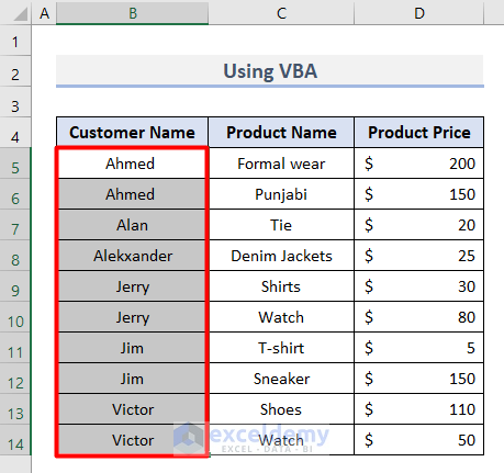
- Press Alt + F11 to open the Microsoft Visual Basics for Applications window.
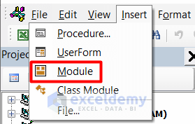
- Choose Module from the Insert tab.
- Copy this code in the Code window.
Option Explicit
Sub MergeSameCells()
Application.DisplayAlerts = False
Dim rg As Range
MergeCells:
For Each rg In Selection
If rg.Value = rg.Offset(1, 0).Value And rg.Value <> "" Then
Range(rg, rg.Offset(1, 0)).Merge
GoTo MergeCells
End If
Next
End Sub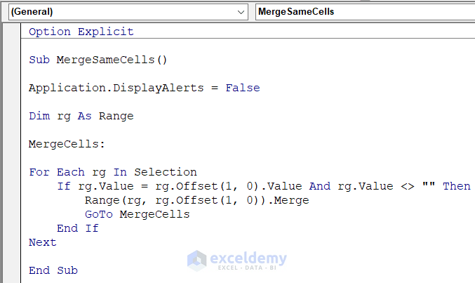
- Press F5 to run the code.
- Click on Run in the Macros window.

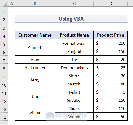
- You will get the merged rows.
Read More: How to Combine Rows with Same ID in Excel
Method 5 – Create a Helper Column to Merge Identical Rows
- Select the cell range B5:B14.
- Select Data and go to Outline, then choose Subtotal.
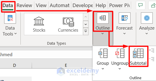
- You will get a warning message window. Click on OK.

- You will get the Subtotal dialogue box.
- Keep the selections as shown below and click on OK.
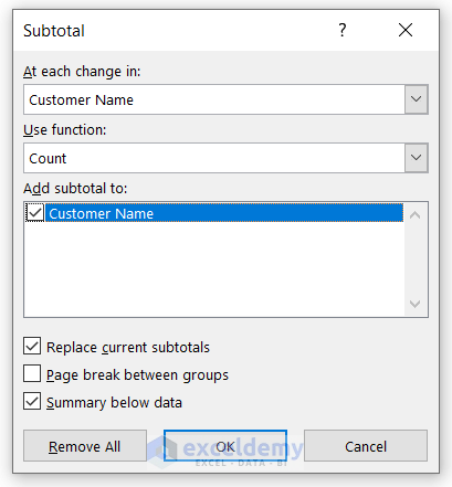
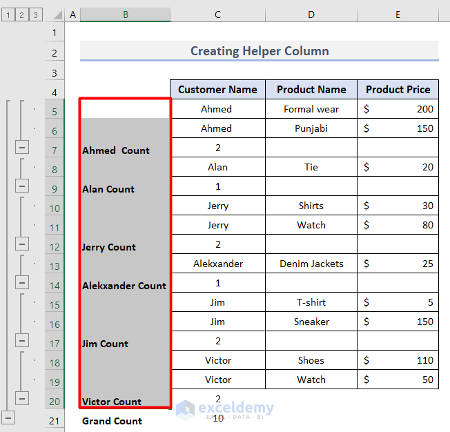
- You will get a helper column next to the original dataset.
- Select the cell range B5:B20.
- Press Ctrl + G on your keyboard to open the Go To window.
- Click on Special.
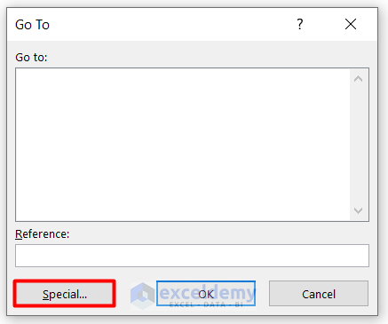
- Select Blanks in the Go To Special window and click on OK.

- All the blank cells will be selected.
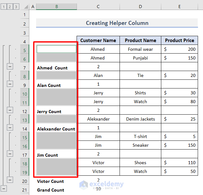
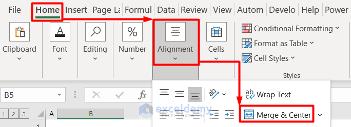
- Select Home, then go to Alignment and choose Merge & Center.
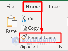
- Choose Format Painter from the Home tab.
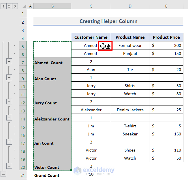
- You will get a Brush icon.
- Hover it through the Customer Name column to match the format of the helper column.
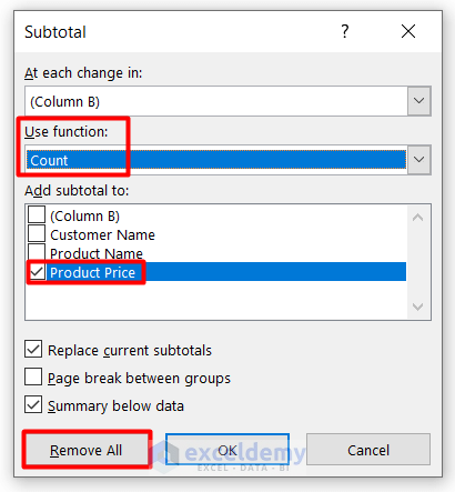
- Open the Subtotal window again.
- Choose Count in the Use function list.
- Choose Product Price under the Add subtotal to box.
- Press Remove All and then delete the helper column.
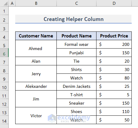
- You will get the merged rows.
Read More: How to Merge Rows in Excel Based on Criteria
Download the Practice Workbook
Further Readings
- How to Combine Multiple Rows into One Cell in Excel
- How to Merge Rows Without Losing Data in Excel
- How to Merge Two Rows in Excel
- How to Merge Rows and Columns in Excel
- How to Merge Rows with Comma in Excel
- How to Convert Multiple Rows to a Single Column in Excel
- How to Convert Multiple Rows to Single Row in Excel
<< Go Back to Merge Rows in Excel | Merge in Excel | Learn Excel
Get FREE Advanced Excel Exercises with Solutions!


Thank you so much for this, saved me a lot of hours of work!
You’re welcome, CHRIS! Best regards!
Very useful. thanks
Merging “visually” (i.e. keeping the value and the sorting/filtering features) same values in column is a feature that has been missing in Excel for many years! About 20 years ago already, I had developped a VBA macro of the kind shown here to merge the cells, but I believe MS should include such feature in the core Excel…
Run time Error ‘1004’ for the line of code
If rg.Value = rg.Offset(1, 0).Value And rg.Value “” Then
what to do next
Hello,
In our Excel file the code is working perfectly without errors.
The possible reasons of getting errors in you end might be: Selecting a range at the edge of the worksheet or having non-contiguous selections.
You can add a check to avoid out-of-bounds errors:
This prevents the code from trying to access an offset that doesn’t exist (the last row in the selection).
Regards
ExcelDemy