How to Apply Number Format in Millions with Comma in Excel (5 Methods)

Method 1 – Using Custom Format to Apply Number Format in Millions with Comma in Excel

1.1 Use of Placeholder Pound (#) Sign

STEPS:

• Select the columns that contain the numbers. We have selected Column C. You can also select a single cell if you have only one large number.

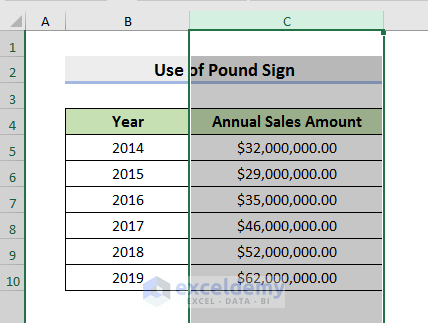
• Press Ctrl + 1 to open the Format Cells window.
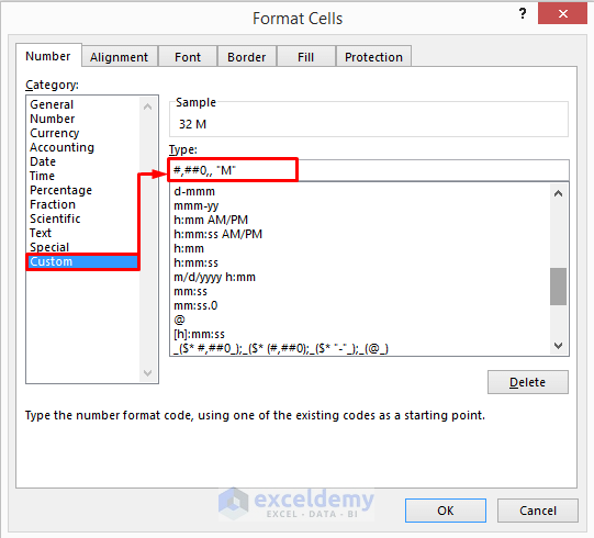
• Select Number and go to Custom.
• Enter the following formula in the Type field.

• Click OK to proceed.

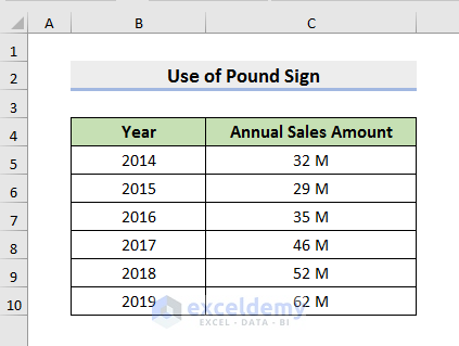
1.2 Use of Placeholder Zero and Decimal Point

STEPS:

• Select Column C.

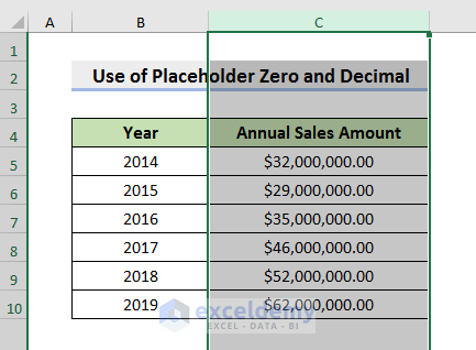
• Press Ctrl + 1. It will open the Format Cells window.
• Select Select Custom.
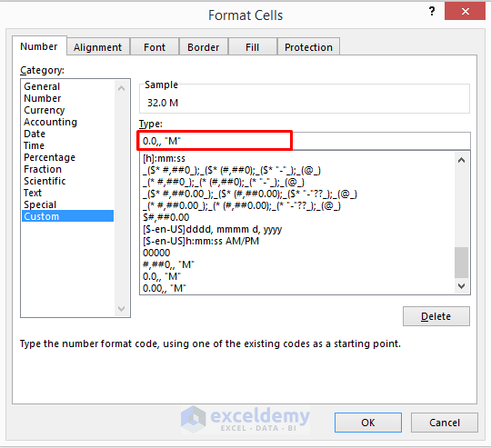
• Enter the following formula in the Type field:

• Click OK to proceed.

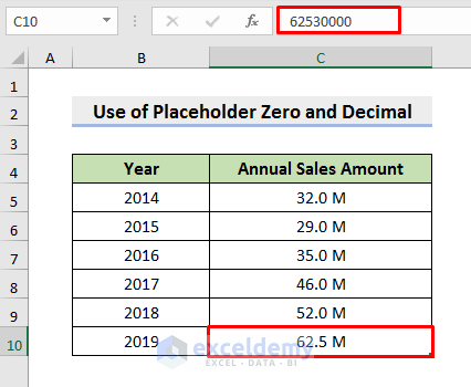
• If you select Cell C10, you can see it displays the value to one decimal point.

• To display the number to two decimal points, enter the following formula in the Type field:

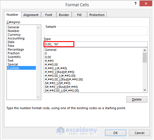
• Click OK.

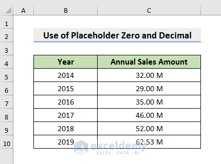
Note:

You may not get the precise value after formatting a number in millions. To fix this, change the decimal points in the Type field of the Format Cells window.

Read More: Excel Custom Number Format – Millions with One Decimal

Method 2 – Setting Number Format in Millions with Comma Using Excel Conditional Formatting

STEPS:

• Select the column that contains the numbers. We have selected Column C.

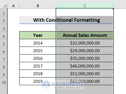
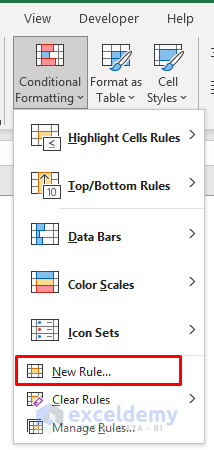
• Go to the Home tab and select Conditional Formatting.

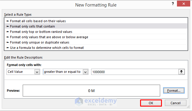
• Select New Rule from the drop-down menu. It will open the New Formatting Rule window.

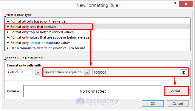
• Select Format only cells that contain.
• Select greater than or equal to and enter 1000000 in the Format only cells with field.
• Select Format. It will open the Format Cells window.

• In the Format Cells window, click Number tab and select Custom.
• Enter the following formula in the Type field:

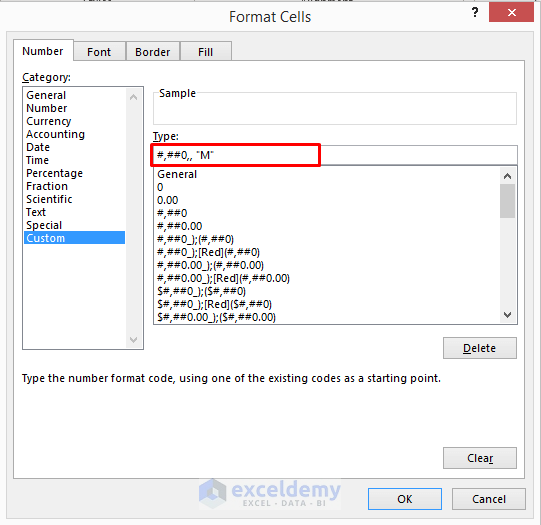
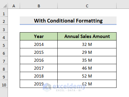
• Click OK to proceed. Click OK in the New Formatting Rule window.

Read More: How to Apply Custom Number Format in Excel with Multiple Conditions

Method 3 – Inserting Excel ROUND Function to Implement Number Format in Millions with Comma

STEPS:

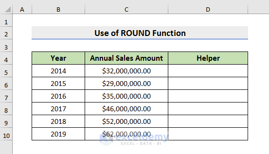
• Create a helper column.

• Select Cell D5 and add the formula:

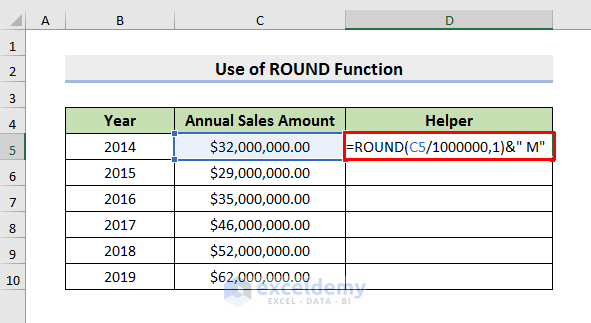
• Press Enter to see the result in Cell D5.

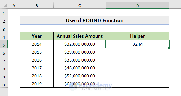
The formula first divides the number of Cell C5 by 1000000 and rounds it up to 1 digit. We have used the ampersand (&) sign to display M which denotes a million.

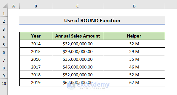
• Drag the Fill Handle down to see results in all cells.

Read More: How to Apply Custom Format Cells in Excel

Method 4 – Using Excel TEXT Function to Apply Number Format in Millions with Comma

STEPS:

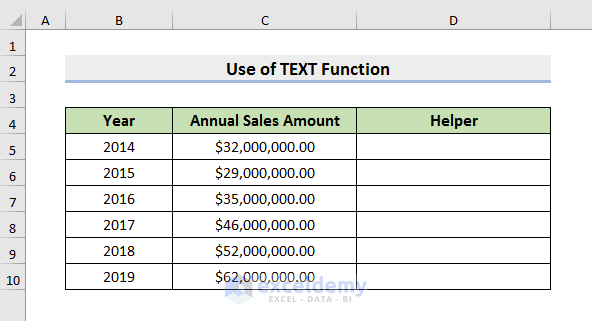
• Create a helper.

• Select Cell D5 and enter the formula:

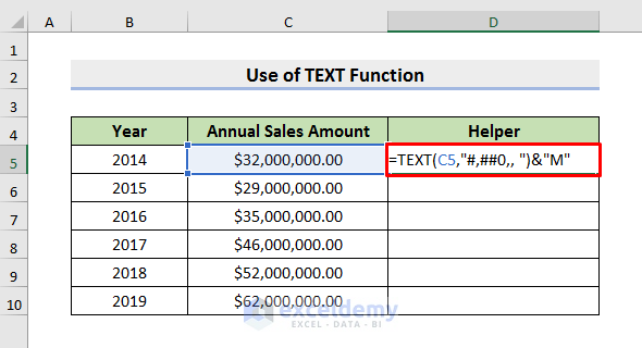
• Press Enter to see the result.

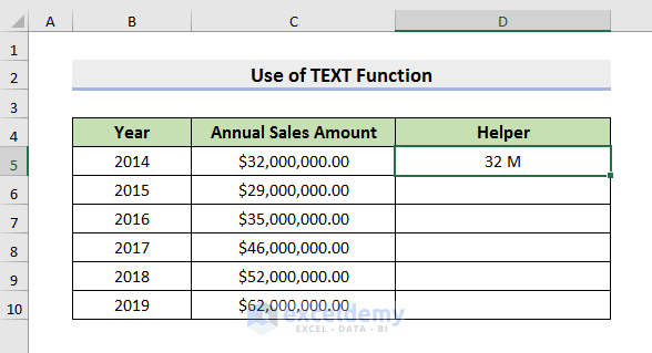
The TEXT function first converts the number of Cell C5 to a text string and formats it as the pound (#) sign. We have used the ampersand (&) sign to display M which denotes a million.

• Use the Fill Handle to see results in all cells.

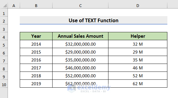
Read More: How to Add Number with Text in Excel Cell with a Custom Format

Method 5 – Using ‘Paste Special’ in Excel to Apply Number Format in Millions with Comma

STEPS:

• Select any cell and enter 1000000. We have selected Cell E5.
• Press Ctrl + C to copy.

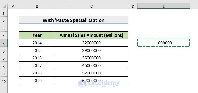
• Select the cells that contain the large numbers.

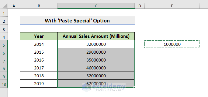
• After selecting the cells, press Ctrl + Alt + V to open the Paste Special window.
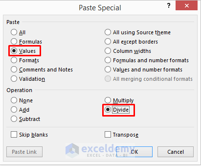
• Select Values in the Paste field and Divide in the Operation field.
• Click OK to proceed.

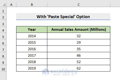
• You will see results as shown in the image below.

Read More: How to Format Numbers to Millions in Excel

Download Practice Book

Related Articles

• How to Format a Number in Thousands K and Millions M in Excel
• How to Add Text after Number with Custom Format in Excel

<< Go Back to Custom Number Format | Number Format | Learn Excel