Method 1 – Using a Formula to Calculate Percentile Rank in Excel
Step-01:
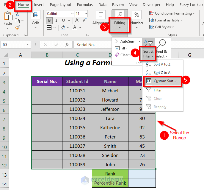
Before adding the serial numbers of these marks we have to sort the marks in Ascending order (from smallest to highest value).
➤ After selecting the range, go to Home Tab >> Editing Group >> Sort & Filter Dropdown >> Custom Sort Option.
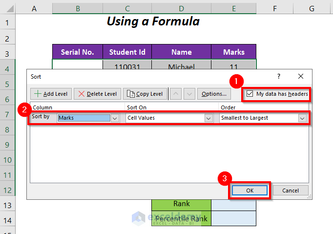
The Sort dialog box will appear.
➤ Check the My data has headers option and select the following
Sort by → Marks (the column name on the basis of which we are sorting)
Sort On → Cell Values
Order → Smallest to Largest
➤ Press OK.
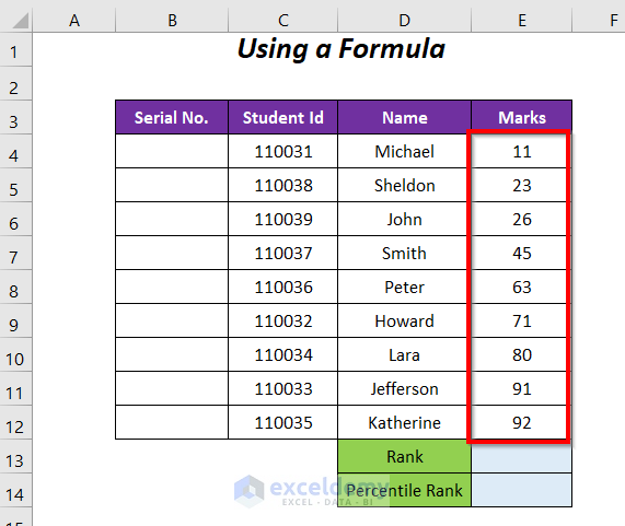
You will get the marks from the lowest value to the highest value.
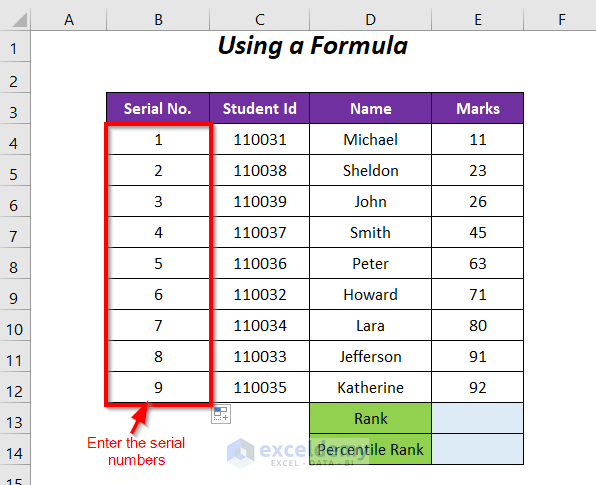
➤ Enter the serial numbers of the marks in the Serial No. column.
Step-02:
We will get the rank of the 65th percentile mark.
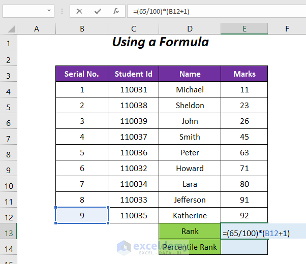
➤ Use the following formula in the cell E13
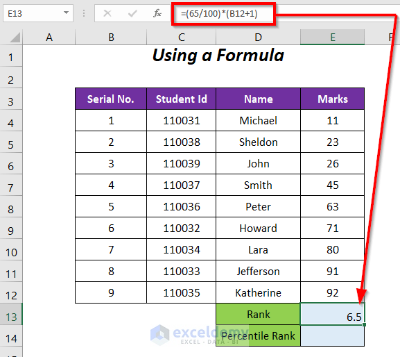
=(65/100)*(B12+1)B12 is the total number of marks and after being added with 1, it will be 10 and we will multiply it with 0.65 (percentile rank).
We are getting 6.5 as the Rank.
We will determine the corresponding marks at the 65th percentile by using the following formula
=E9+(E13-B9)*(E10-E9)E9 is the marks at serial number 6, E10 is the marks at serial number 7, E13 is the Rank, and B9 is the serial number 6.
(E13-B9)→ 6.5-6
Output → 0.5
(E10-E9)→ 80-71
Output → 9
E9+(E13-B9)*(E10-E9)becomes
71+0.5*9
Output → 75.5
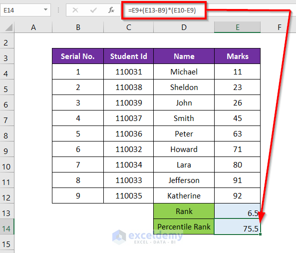
We are getting the marks 75.5 as 65th percentile mark which is in between the marks of serial numbers 6 and 7.
Method 2 – Combining RANK.EQ and COUNT Function to Calculate Percentile Rank
Steps:
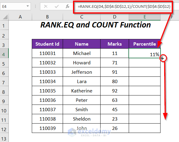
➤ Type the following formula in the cell E4
=RANK.EQ(D4,$D$4:$D$12,1)/COUNT($D$4:$D$12)D4 is the marks for the student Michael, $D$4:$D$12 is the range of marks and 1 is the Ascending Order (it will return 1 for the lowest mark and the highest rank for the highest number).
EQ(D4,$D$4:$D$12,1)→ determines the rank of the mark in cell D4 among the range of the marks $D$4:$D$12.
Output → 1 (as the number in the cell D4 is the lowest number in the range)
COUNT($D$4:$D$12)→ counts the number of non-blank cells in this range
Output → 9
EQ(D4,$D$4:$D$12,1)/COUNT($D$4:$D$12)becomes
1/9
Output → 0.11 or 11%
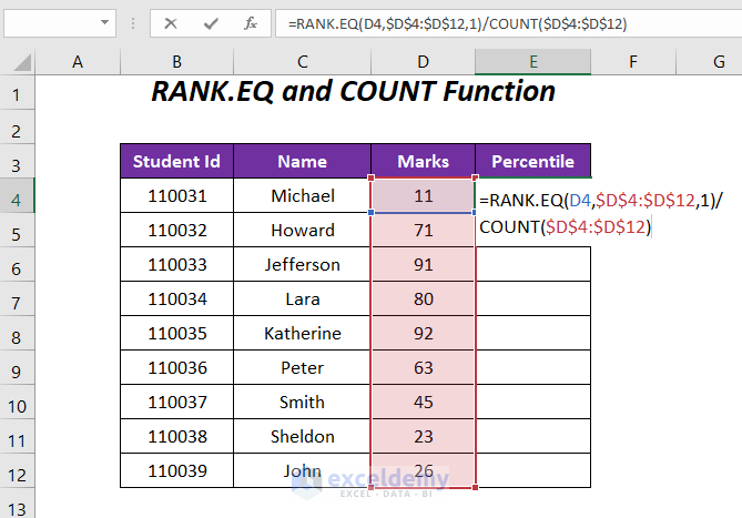
➤ Press ENTER and drag down the Fill Handle tool.
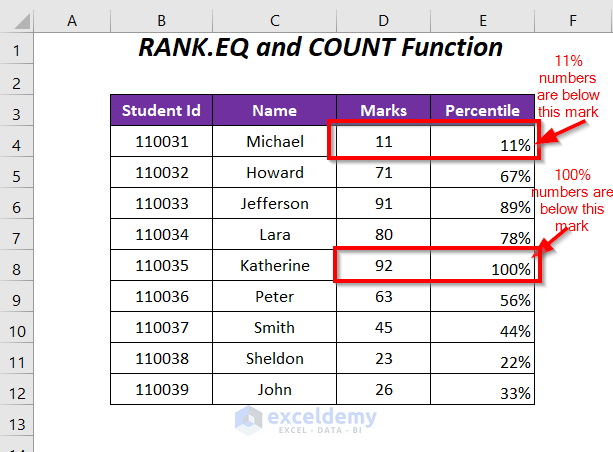
Result:
We will get the percentile ranks of the marks; for example, the lowest rank 11%, means there are only 11% marks below this mark and (100-11)% or 89% marks are above this mark, 100% means 100% marks are below this mark and (100-100)% or 0% marks are above this mark.
Method 3 – Using PERCENTRANK.INC Function to Calculate Percentile Rank in Excel
Steps:
➤ Type the following formula in the cell E4:
=PERCENTRANK.INC($D$4:$D$12,D4)D4 is the marks for the student Michael, $D$4:$D$12 is the range of marks.
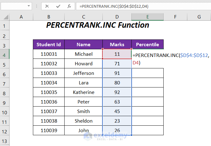
➤ Press ENTER and drag down the Fill Handle tool.
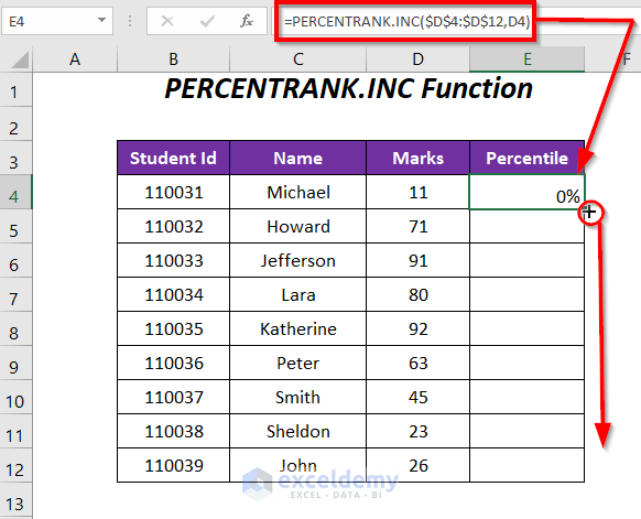
Result:
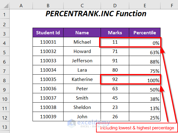
We are getting 0% for the lowest mark, which means there are no marks below this mark, and 100% for the highest mark, which means all of the marks are below this mark.
Method 4 – Using Excel PERCENTRANK.EXC Function to Calculate Percentile Rank
Steps:
➤ Type the following formula in the cell E4
=PERCENTRANK.EXC($D$4:$D$12,D4)D4 is the marks for the student Michael, $D$4:$D$12 is the range of marks.
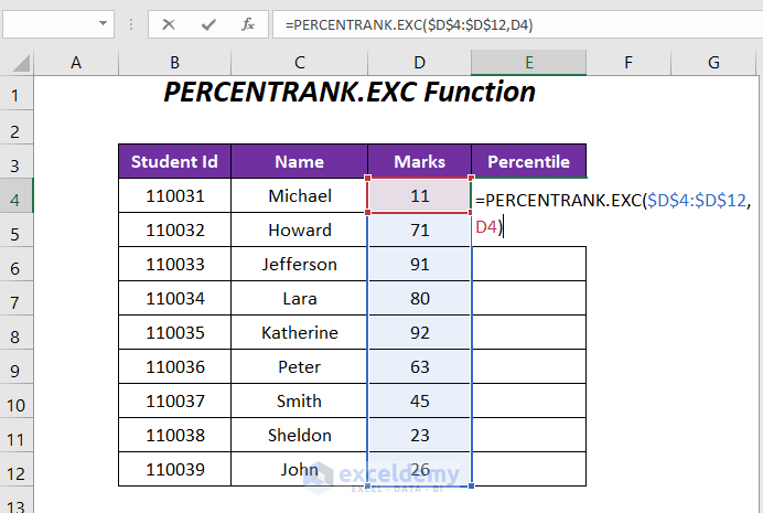
➤ Press ENTER and drag down the Fill Handle tool.
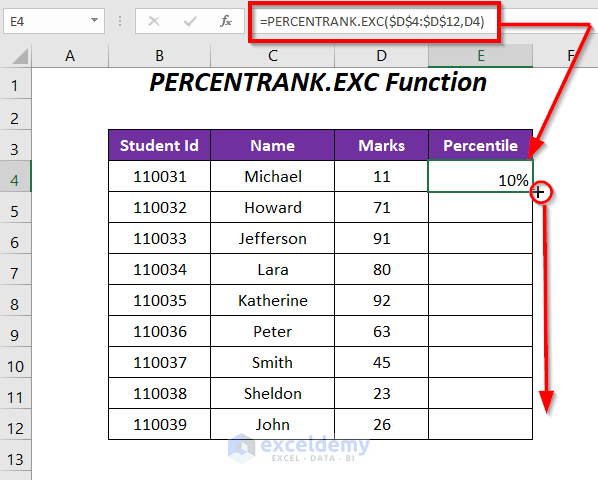
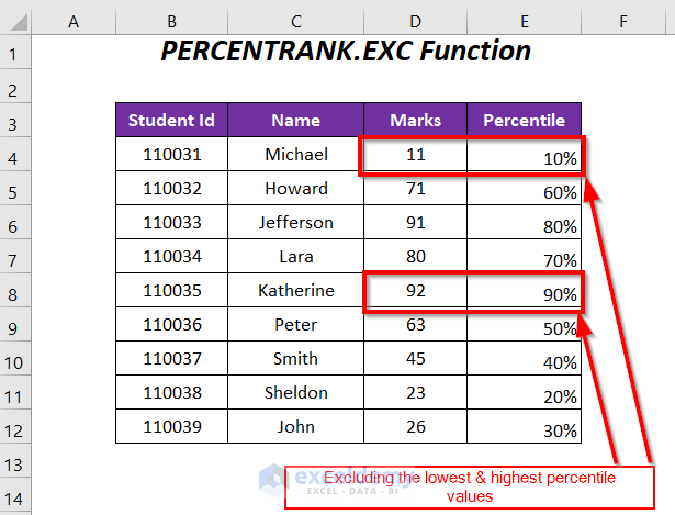
Result:
We are getting 10% for the lowest mark instead of 0% and 90% for the highest mark in lieu of 100%.
Method 5 – Using PERCENTILE.INC Function
Steps:
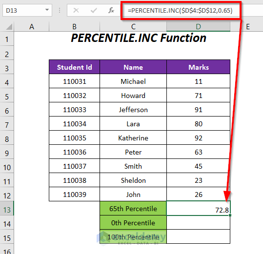
➤ Type the following formula in the cell D13
=PERCENTILE.INC($D$4:$D$12,0.65)$D$4:$D$12 is the range of marks, and 0.65 is for the 65th percentile.
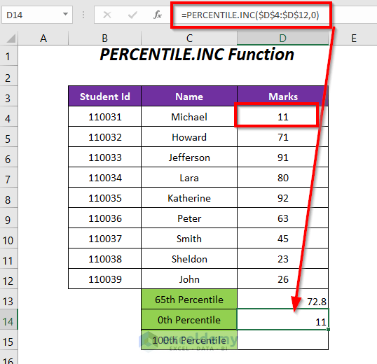
To get the mark at the 0th percentile, enter the following formula in the cell D14:
=PERCENTILE.INC($D$4:$D$12,0)$D$4:$D$12 is the range of marks, and 0 is for the 0th percentile.
It is returning the lowest mark of the range for the 0th percentile.
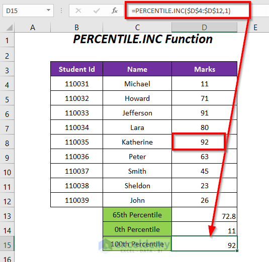
Use the following formula in the cell D15 to have the mark at the 100th percentile rank
=PERCENTILE.INC($D$4:$D$12,1)$D$4:$D$12 is the range of marks, and 1 is for the 100th percentile.
It is returning the highest mark of the mange for the 100th percentile.
Method 6 – Using PERCENTILE.EXC Function to Calculate Percentile Rank in Excel
Steps:
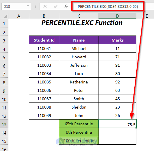
➤ Type the following formula in the cell D13:
=PERCENTILE.EXC($D$4:$D$12,0.65)$D$4:$D$12 is the range of marks, and 0.65 is for the 65th percentile.
To get the mark at the 0th percentile, enter the following formula in the cell D14
=PERCENTILE.EXC($D$4:$D$12,0)Here, $D$4:$D$12 is the range of marks, and 0 is for the 0th percentile.
It is returning the #NUM! error because of the PERCENTILE.EXC function will work with the values excluding the bottom value of the range.
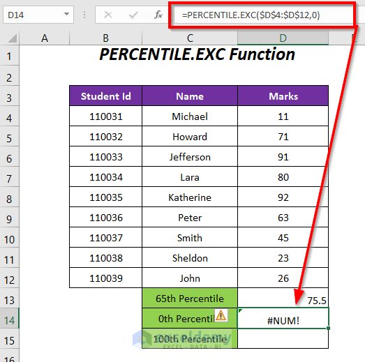
To have the mark at the 100th percentile, enter the following formula in the cell D15:
=PERCENTILE.EXC($D$4:$D$12,1)$D$4:$D$12 is the range of marks, and 1 is for the 100th percentile.
It is returning the #NUM! error because of the PERCENTILE.EXC function will work with the values excluding the top value of the range.
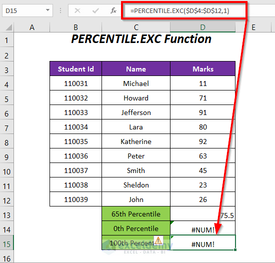
To avoid the #NUM! error, you have to be careful that you can’t use 0 and 1 for determining the lowest and highest marks; you can use 0.1 instead of 0 and 0.9 instead of 1.
Method 7 – Using SUMPRODUCT and COUNTIF Functions for Conditional Ranking
Steps:
➤ Type the following formula in the cell E4
=SUMPRODUCT(($B$4:$B$12=B4)*(D4>$D$4:$D$12))/COUNTIF($B$4:$B$12,B4)D4 is the marks for the student Michael, $D$4:$D$12 is the range of marks, B4 is the name of the student, and $B$4:$B$12 is the range of names.
SUMPRODUCT(($B$4:$B$12=B4)*(D4>$D$4:$D$12))becomes
SUMPRODUCT(({TRUE;FALSE;TRUE;FALSE;TRUE;FALSE;FALSE;FALSE;FALSE})*({FALSE;FALSE;FALSE;FALSE;FALSE;FALSE;FALSE;FALSE;FALSE}))→SUMPRODUCT({0;0;0;0;0;0;0;0;0})
Output → 0
COUNTIF($B$4:$B$12, B4)→ counts the number of presence of the student Michael in the Name column
Output → 3
SUMPRODUCT(($B$4:$B$12=B4)*(D4>$D$4:$D$12))/COUNTIF($B$4:$B$12,B4)becomes
0/3
Output → 0%
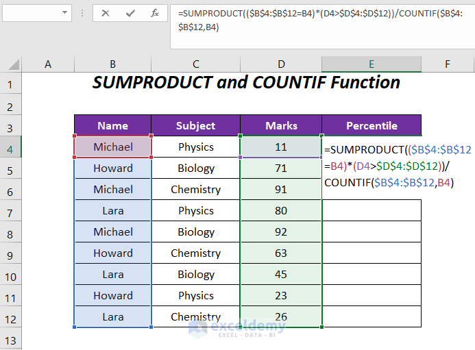
➤ Press ENTER and drag down the Fill Handle tool.
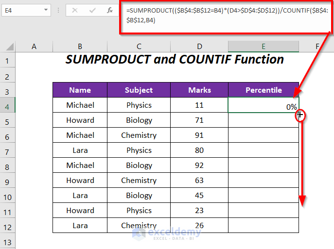
Result:
We have different percentile rankings for the three subjects for different students: the Red indicating box is for Michael, the Blue indicating box is for Howard, and the Green indicating box is for Lara.

Download Workbook
Related Articles
- How to Rank Average in Excel
- How to Rank in Excel Highest to Lowest
- How to Stack Rank Employees in Excel
- How to Create a Ranking Graph in Excel
- How to Create an Auto Ranking Table in Excel
<< Go Back to Excel RANK Function | Excel Functions | Learn Excel
Get FREE Advanced Excel Exercises with Solutions!

